Visualization and Summary Statistics
UCLA Soc 114
Review of last class
Say this code in English:
numbers <- c(1,2,3)
x_length <- length(numbers)
- Store the vector
c(1,2,3) in the object numbers
- Use the
length() function to get the length of numbers
Learning goals for today
- Reason about distributions
- and visualize with
ggplot()
- Understand summary statistics
- and construct with
summarize()
- Write clean code with the pipe
|>
How to visualize?
How might we visualize the U.S. income distribution?
Here are some data:
library(tidyverse)
incomeSimulated <- read_csv(
  file = "https://soc114.github.io/data/incomeSimulated.csv"
)
# A tibble: 1,000 × 2
     id hhincome
  <dbl>    <dbl>
1     1   19170.
2     2  124474.
3     3   25114.
# ℹ 997 more rows
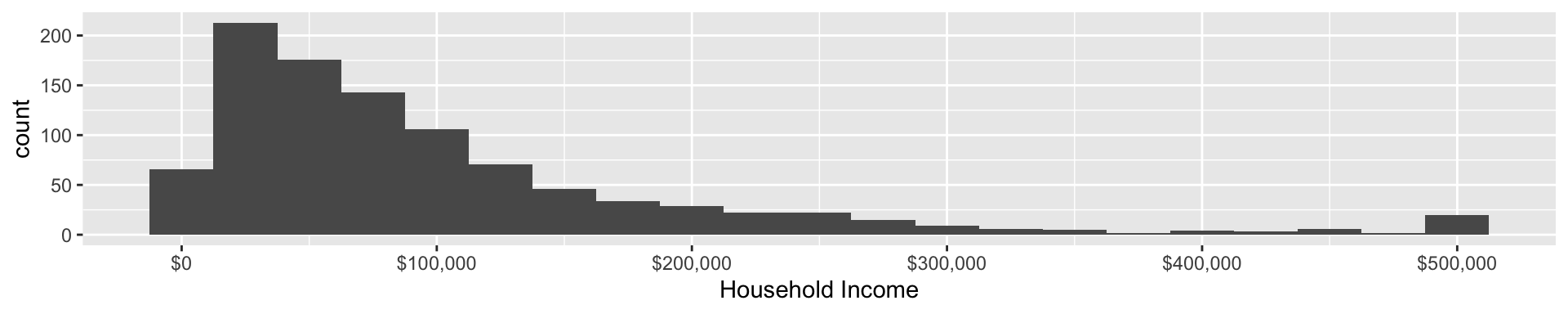
Visualize with a histogram
![]()
- Bins of $25,000
- In each bin, count number of people
Learning a new function: ggplot
ggplot(
  data = incomeSimulated,
  mapping = aes(x = hhincome)
)
![]()
Two arguments get us started:
data argument contains datamapping argument maps data to plot elements
Within mapping,
aes() defines the aesthetics of the plot- i.e. which variable goes along x-axis
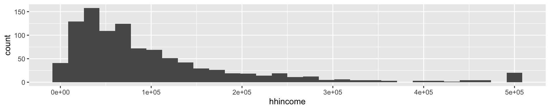
Adding a layer: geom_histogram()
ggplot(
  data = incomeSimulated,
  mapping = aes(x = hhincome)
) +
  geom_histogram()
![]()
- The
+ indicates that a new layer is coming
geom_histogram() is the new layer- Inherits the
data and mapping of the plot
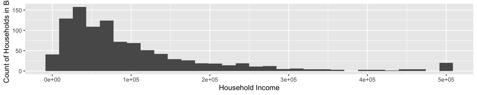
Update axis titles
ggplot(
  data = incomeSimulated,
  mapping = aes(x = hhincome)
) +
  geom_histogram() +
  labs(
    x = "Household Income",
    y = "Count of Households in Bin"
  )
![]()
Learning goals for today
- Reason about distributions
- and visualize with
ggplot()
- Understand summary statistics
- and construct with
summarize()
- Write clean code with the pipe
|>
Imagine 3 income distributions
| 1 |
$10k |
$40k |
$50k |
| 2 |
$60k |
$65k |
$60k |
| 3 |
$150k |
$70k |
$65k |
Normative question: Which one is better?
Summary statistic
A summary statistic aggregates a distribution to one number
For example, the mean \[\text{mean}(\vec{x}) = \frac{x_1 + x_2 +\cdots}{n}\]
Summary statistic: Mean
| 1 |
$10k |
$40k |
$50k |
| 2 |
$60k |
$65k |
$60k |
| 3 |
$150k |
$70k |
$65k |
| Mean |
$73k |
$58k |
$58k |
By the mean, Distribution 1 seems the best.
Summary statistic: Minimum
Find the lowest value.
| 1 |
$10k |
$40k |
$50k |
| 2 |
$60k |
$65k |
$60k |
| 3 |
$150k |
$70k |
$65k |
Summary statistic: Minimum
Find the lowest value.
| 1 |
$10k |
$40k |
$50k |
| 2 |
$60k |
$65k |
$60k |
| 3 |
$150k |
$70k |
$65k |
| Minimum |
$10k |
$40k |
$50k |
By the minimum, Distribution 3 seems the best.
Which summary statistic to choose?
Minimum? Median? Mean?
| 1 |
$10k |
$40k |
$50k |
| 2 |
$60k |
$65k |
$60k |
| 3 |
$150k |
$70k |
$65k |
Choosing a summary statistic
Which summary to choose is not an empirical question.
- Depends on what aspect of the distribution matters to you
The value of a chosen summary statistic is empirical.
- Data can tell us a value for the mean, the median, the minimum, etc.
The summarize() function
The summarize() function aggregates data to summaries.
- Input is a dataset with \(n\) rows
- Output is a summary with 1 row
The summarize() function
# A tibble: 1,000 × 2
     id hhincome
  <dbl>    <dbl>
1     1   19170.
2     2  124474.
3     3   25114.
# ℹ 997 more rows
The summarize() function
summarize(
  .data = incomeSimulated,
  estimated_mean = mean(hhincome)
)
# A tibble: 1 × 1
  estimated_mean
           <dbl>
1        100899.
.data is input dataestimated_mean is a variable in output datamean(hhincome) is the mean household income
The summarize() function: Several summaries
summarize(
  .data = incomeSimulated,
  estimated_mean = mean(hhincome),
  estimated_median = median(hhincome),
  esitmated_min = min(hhincome)
)
# A tibble: 1 × 3
  estimated_mean estimated_median esitmated_min
           <dbl>            <dbl>         <dbl>
1        100899.           69035.             0
Learning goals for today
- Reason about distributions
- and visualize with
ggplot()
- Understand summary statistics
- and construct with
summarize()
- Write clean code with the pipe
|>
Piping code with |>
The pipe |> passes x as the first argument to the length() function.
Piping code with |>
Stylistically helpful
- Data is a different kind of argument
- Pipes will help us in the future
incomeSimulated |>
  summarize(
    estimated_mean = mean(hhincome),
    estimated_median = median(hhincome),
    esitmated_min = min(hhincome)
  )
# A tibble: 1 × 3
  estimated_mean estimated_median esitmated_min
           <dbl>            <dbl>         <dbl>
1        100899.           69035.             0
Learning goals for today
- Reason about distributions
- and visualize with
ggplot()
- Understand summary statistics
- and construct with
summarize()
- Write clean code with the pipe
|>
You can now learn more: R4DS Ch 1 and Ch 3