# A tibble: 10 × 3
  player          team          salary
  <chr>           <chr>          <dbl>
1 Matz, Steven    St. Louis   10500000
2 Barlow, Scott   Kansas City  5300000
3 Pomeranz, Drew* San Diego   10000000
# ℹ 7 more rows
# A tibble: 3 × 3
  player              team       salary
  <chr>               <chr>       <dbl>
1 Houck, Tanner       Boston     740000
2 Gallegos, Giovanny  St. Louis 4750000
3 Hernandez, Jonathan Texas      995000
# A tibble: 3 × 3
  player             team       salary
  <chr>              <chr>       <dbl>
1 Gallegos, Giovanny St. Louis 4750000
2 Gallegos, Giovanny St. Louis 4750000
3 Houck, Tanner      Boston     740000
# A tibble: 3 × 3
  player              team       salary
  <chr>               <chr>       <dbl>
1 Gallegos, Giovanny  St. Louis 4750000
2 Hernandez, Jonathan Texas      995000
3 Gallegos, Giovanny  St. Louis 4750000
# A tibble: 3 × 3
  player              team  salary
  <chr>               <chr>  <dbl>
1 Hernandez, Jonathan Texas 995000
2 Hernandez, Jonathan Texas 995000
3 Hernandez, Jonathan Texas 995000
# A tibble: 3 × 3
  player             team       salary
  <chr>              <chr>       <dbl>
1 Houck, Tanner      Boston     740000
2 Gallegos, Giovanny St. Louis 4750000
3 Gallegos, Giovanny St. Louis 4750000
Coding concepts
We will analyze hundreds of bootstrap samples.
We need two coding concepts.
How to write an estimator function
How to write a for loop
How to write an estimator function
A function (like mean) takes an input and returns an output. You can write your own.
estimator <-function(data) { data |>summarize(estimate =mean(salary)) |>pull(estimate)}
The function takes data and returns an estimate.
estimator(data = sampled_players)
[1] 6254938
How to write a for loop
Useful for tasks you will repeat.
First, initialize a vector to hold results.
vector_for_results <-rep(NA, 3)
The rep function repeates the value NA 3 times.
Second, loop through and fill your vector.
for (index in1:3) { vector_for_results[index] <- index}
Square brackets [] extract an element of a vector.
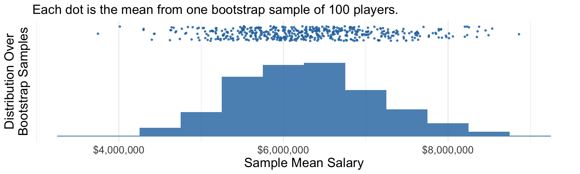
Analyze 500 bootstrap samples
Initialize a vector to hold the result.
bootstrap_estimates <-rep(NA, times =500)
Analyze 500 bootstrap samples
Write a for loop that will repeat 500 times.
for (index in1:500) {# Draw a bootstrap sample bootstrap_sample <- sampled_players |>slice_sample(prop =1, replace =TRUE)# Construct an estimate estimate_this_index <-estimator(bootstrap_sample)# Store that estimate bootstrap_estimates[index] <- estimate_this_index}
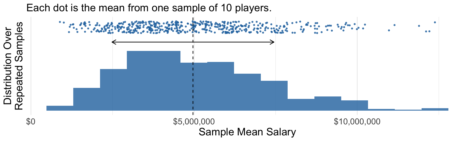
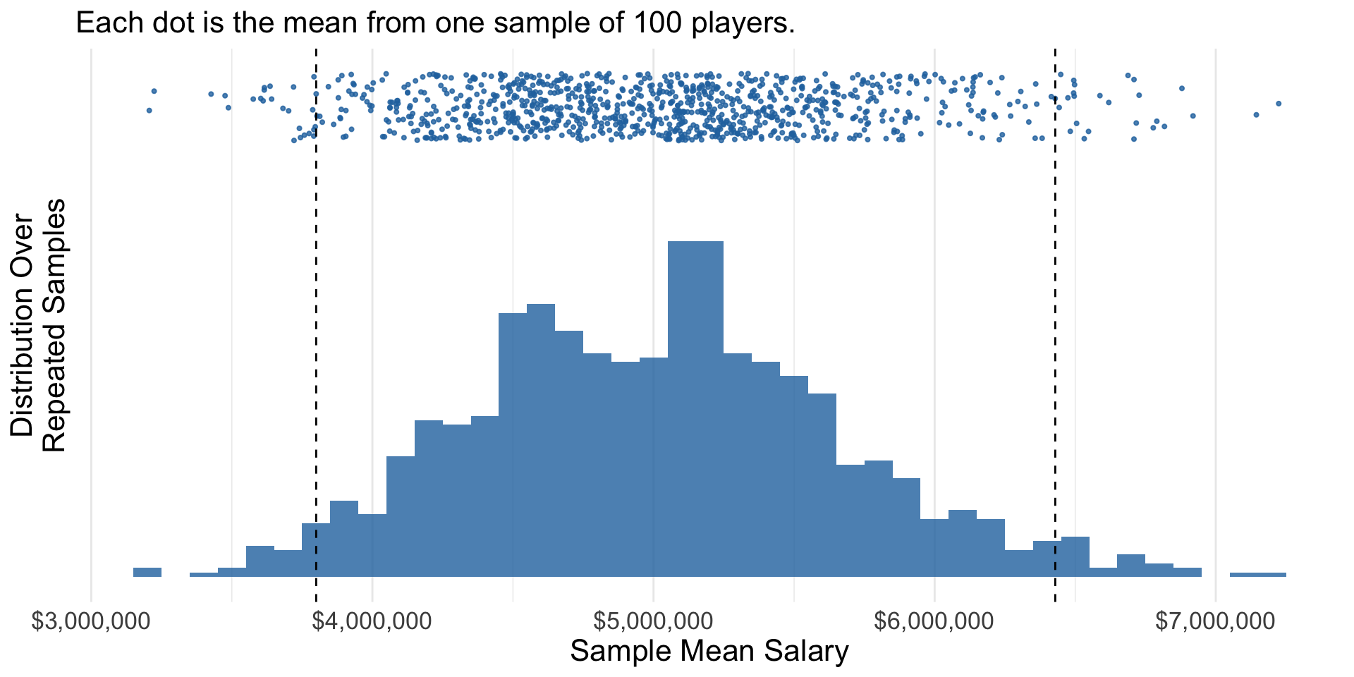
An interval from \(\text{lower}(\text{sample})\) to \(\text{upper}(\text{sample})\) with the property: across repeated samples, 95% of intervals constructed this way would contain the population parameter.
Confidence interval: Example
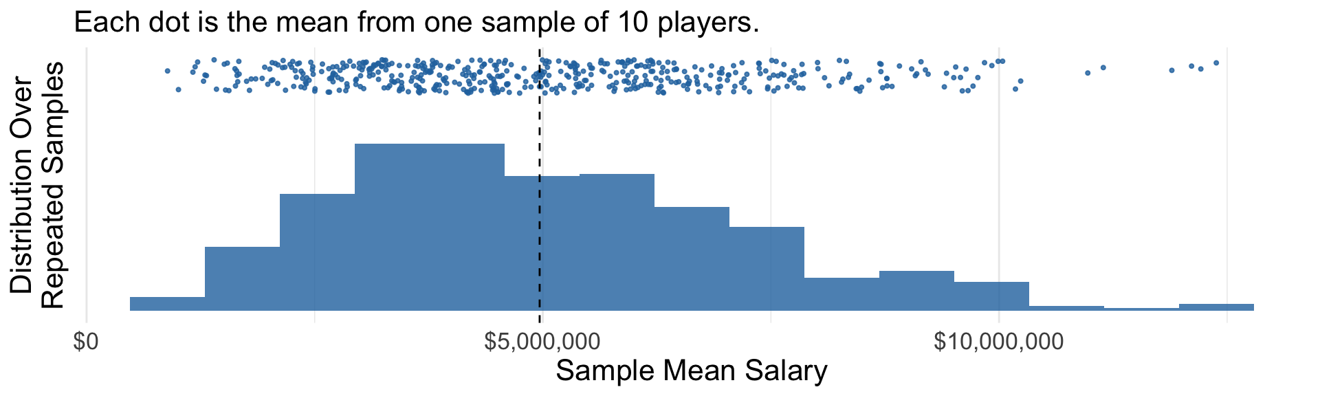
Middle 95% of bootstrap estimates is a confidence interval.