Linear Regression

UCLA Soc 114

Linear regression: Learning goals

Some things you may know

How to fit a linear model
How to make predictions

Data science ideas

Why model at all?
Penalized linear regression

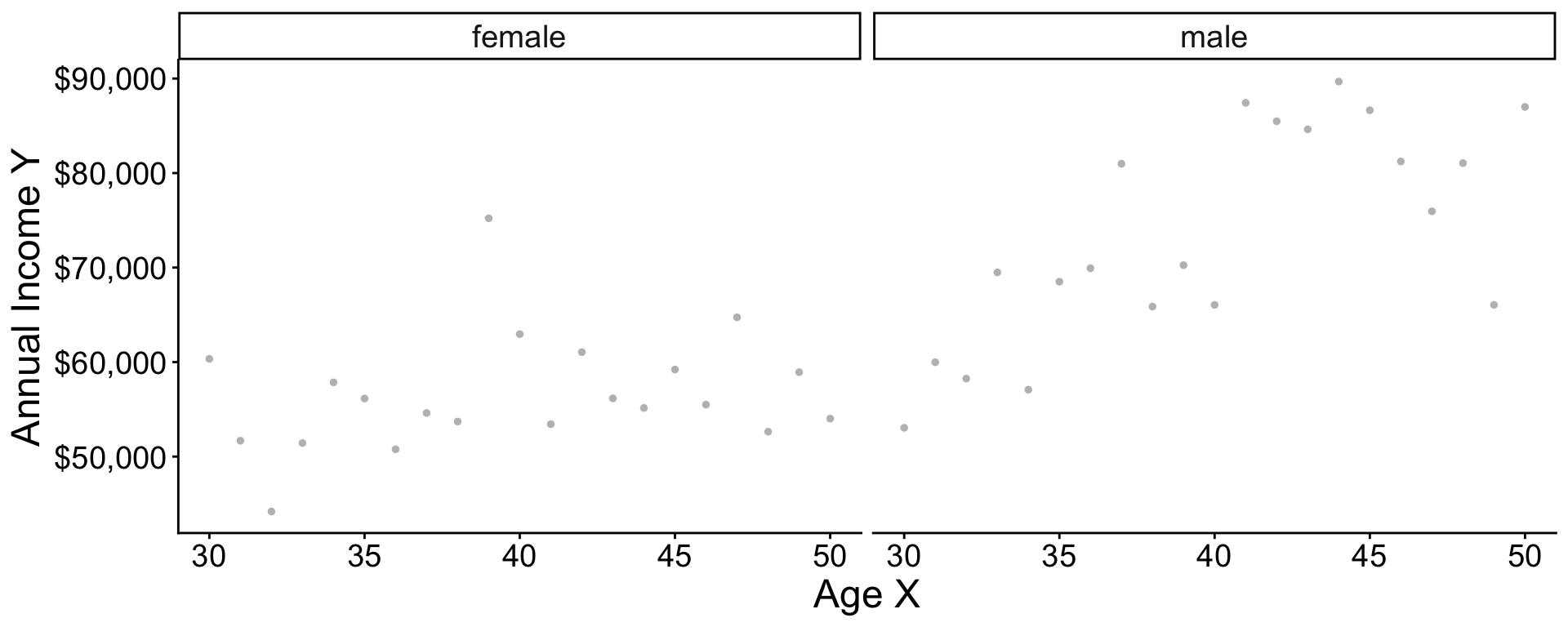
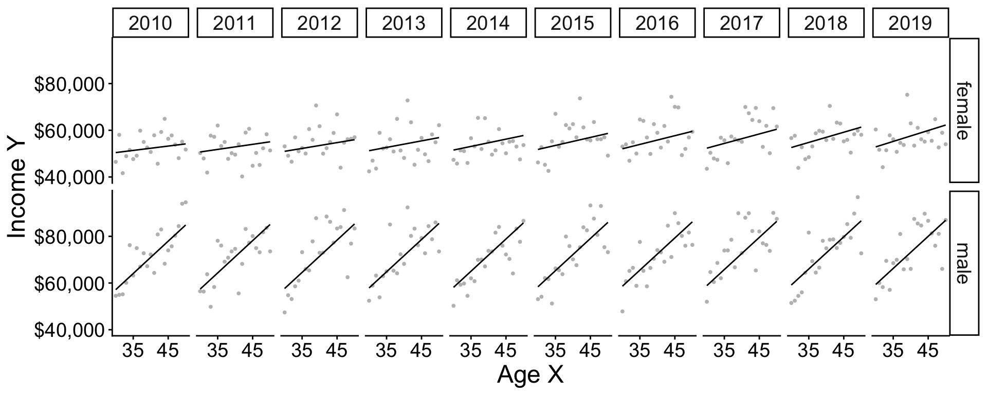
Data for illustration

U.S. adult income by

sex (male, female)
age (30–50)
year (2010–2019)

among those working 35+ hours per week for 50+ weeks per year. Data are simulated based on the 2010–2019 American Community Survey (ACS).

Data for illustration

The function below will simulate data

simulate <- function(n = 100) {
  read_csv("https://ilundberg.github.io/description/assets/truth.csv") |>
    slice_sample(n = n, weight_by = weight, replace = T) |>
    mutate(income = exp(rnorm(n(), meanlog, sdlog))) |>
    select(year, age, sex, income)
}

Data for illustration

simulated <- simulate(n = 3e4)

# A tibble: 30,000 × 4
   year   age sex    income
  <dbl> <dbl> <chr>   <dbl>
1  2011    48 female 93676.
2  2012    38 female 98805.
3  2013    38 female 52330.
# ℹ 29,997 more rows

Conditional expectation

Mean of an outcome within a population subgroup.

expectation refers to taking a mean

conditional refers to within a subgroup

Example: Mean income among females age 47 in 2019

Task. Estimate this in our data.

Code: Find the subgroup

filter() restricts our data to cases meeting requirements:

the sex variable equals the value female
the age variable equals the value 47
the year variable equals the value 2019

subgroup <- simulated |>
  filter(sex == "female") |>
  filter(age == 47) |>
  filter(year == 2019)

Code: Estimate the mean

summarize() aggregates to the mean

subgroup |>
  summarize(conditional_expectation = mean(income))

# A tibble: 1 × 1
  conditional_expectation
                    <dbl>
1                  71530.

Code: Mean in many subgroups

With group_by, you can summarize many subgroups

simulated |>
  group_by(sex, age, year) |>
  summarize(conditional_expectation = mean(income))

# A tibble: 420 × 4
# Groups:   sex, age [42]
  sex      age  year conditional_expectation
  <chr>  <dbl> <dbl>                   <dbl>
1 female    30  2010                  45928.
2 female    30  2011                  43688.
3 female    30  2012                  42714.
# ℹ 417 more rows

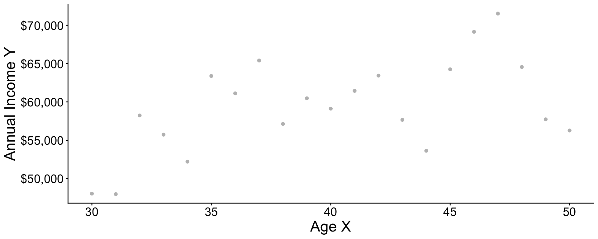
Conditional expectation: Math

The conditional expectation function is the subgroup mean of \(Y\) within a subgroup with the predictor values \(\vec{X} = \vec{x}\).

\[ f(\vec{x}) = \text{E}(Y\mid\vec{X} = \vec{x}) \]

To learn \(f(\vec{x})\) from data is a central task in statistical learning.

Statistical Learning by Pooling Information

A subgroup is small

simulated |>
  filter(sex == "female") |>
  filter(year == 2019) |>
  filter(age == 47)

# A tibble: 67 × 4
   year   age sex    income
  <dbl> <dbl> <chr>   <dbl>
1  2019    47 female 15761.
2  2019    47 female 32995.
3  2019    47 female 83967.
# ℹ 64 more rows

Very few cases \(\rightarrow\) statistically uncertain

How to better estimate for 47-year-old females in 2019?

Pooling information across subgroups

We have many female respondents in 2019. Few are age 47.

simulated |>
  filter(sex == "female") |>
  filter(year == 2019)

# A tibble: 1,427 × 4
   year   age sex    income
  <dbl> <dbl> <chr>   <dbl>
1  2019    32 female 52130.
2  2019    46 female 17465.
3  2019    41 female 66012.
# ℹ 1,424 more rows

Could we use them to learn about the 47-year-olds?

Pooling information across subgroups

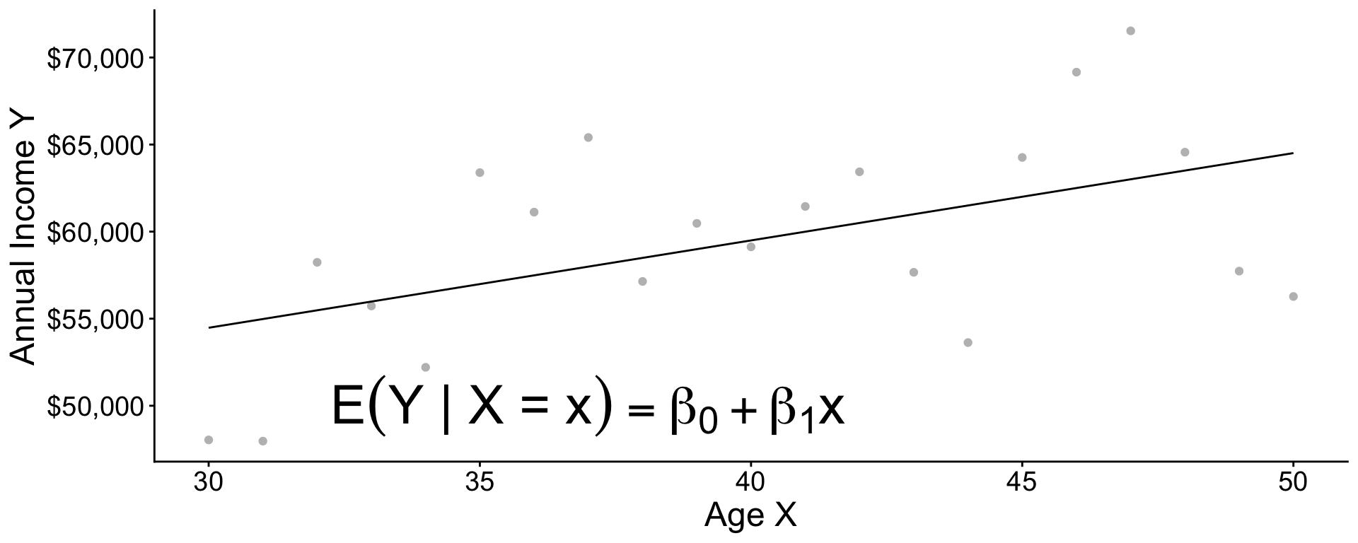
Practice question

\[ \text{E}(Y\mid X) = \beta_0 + \beta_1 X \]

Suppose \(\beta_0 = 5\) and \(\beta_1 = 3\)

What is the conditional mean when \(X = 0\)?
What is the conditional mean when \(X = 1\)?
What is the conditional mean when \(X = 2\)?
How much does the conditional mean change for each unit increase in \(X\)?

Code

The next slides explain how to code a model in R.

Code: Simulate data

Generate some data

simulated <- simulate(n = 3e4)

Restrict to female respondents in 2019

female_2019 <- simulated |>
  filter(sex == "female") |>
  filter(year == 2019)

(Below is simulate if you did not copy it before)

simulate <- function(n = 100) {
  read_csv("https://ilundberg.github.io/description/assets/truth.csv") |>
    slice_sample(n = n, weight_by = weight, replace = T) |>
    mutate(income = exp(rnorm(n(), meanlog, sdlog))) |>
    select(year, age, sex, income)
}

Code: Learn a model

model <- lm(
  formula = income ~ age, 
  data = female_2019
)

model is an object of class lm for linear model
lm() function creates this object
formula argument is a model formula
- outcome ~ predictor is the syntax
data is a dataset containing outcome and predictor

Code: Examine the learned model

summary(model)


Call:
lm(formula = income ~ age, data = female_2019)

Residuals:
   Min     1Q Median     3Q    Max 
-52689 -29518 -12682  16013 400507 

Coefficients:
            Estimate Std. Error t value Pr(>|t|)    
(Intercept)  47242.6     7518.3   6.284 4.37e-10 ***
age            233.7      185.7   1.259    0.208    
---
Signif. codes:  0 '***' 0.001 '**' 0.01 '*' 0.05 '.' 0.1 ' ' 1

Residual standard error: 43360 on 1437 degrees of freedom
Multiple R-squared:  0.001102,  Adjusted R-squared:  0.0004064 
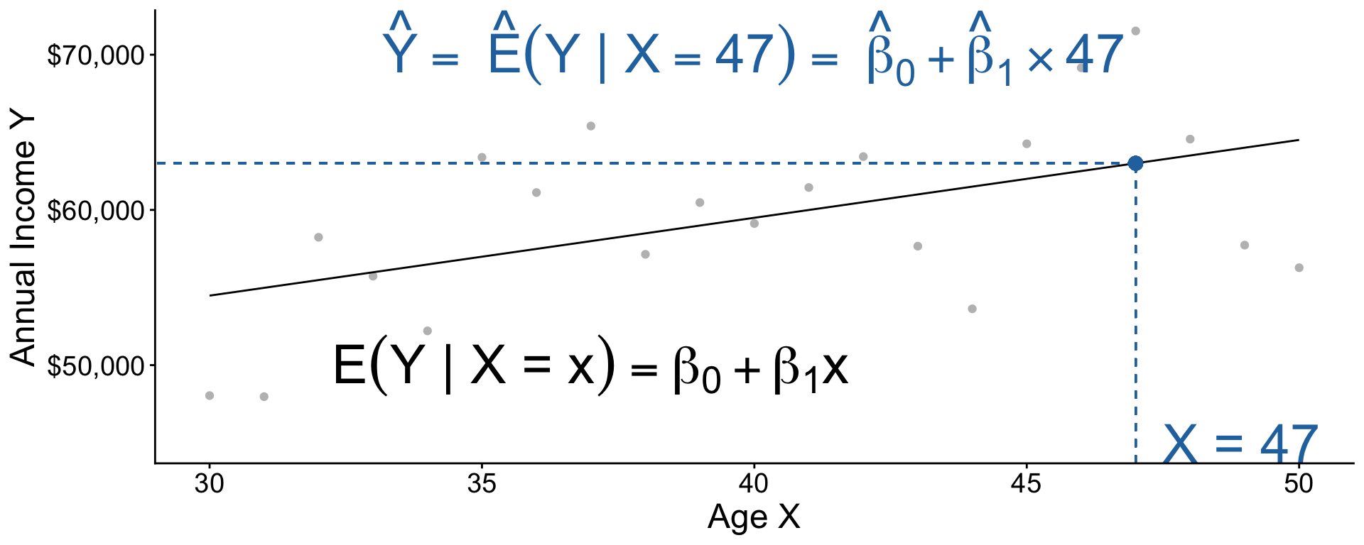
F-statistic: 1.585 on 1 and 1437 DF,  p-value: 0.2083

Code: Predict for a new X value

Define X value at which to predict

to_predict <- tibble(age = 47)

Predict for that subgroup

predict(model, newdata = to_predict)

       1 
58228.57

Recap: Our model pooled information:

People of all ages contributed to model
Then we predicted at a single age

Code: Three steps

Estimate a model
Define \(x\) to predict
Predict \(\hat{Y} = \hat{\text{E}}(Y\mid X = x)\)

What if you were going to do this many times on different data?

Code: Three steps in a function

estimator <- function(data) {
  # Learn the model from the data
  model <- lm(formula = income ~ age, data = data)
  # Define our target subgroup
  to_predict <- tibble(age = 47)
  # Predict
  estimate <- predict(model, newdata = to_predict)
  # Return the estimate
  return(estimate)
}

Code: All together

estimator(data = female_2019)

       1 
58228.57

female_2019 |>
  estimator()

       1 
58228.57

simulated |> 
  filter(sex == "female") |>
  filter(year == 2010) |>
  estimator()

      1 
54637.9

Practice question

Below is the line fit to the population data. Suppose we want to learn \(\text{E}(\log(Y)\mid X = 30)\).

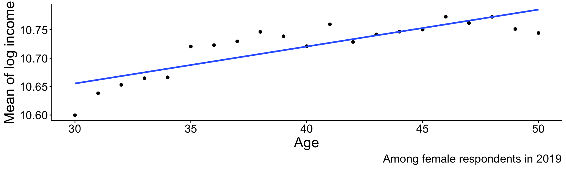
Why might this model make a misleading estimate?
Why might the model still be useful?

Additive vs Interactive

Two models

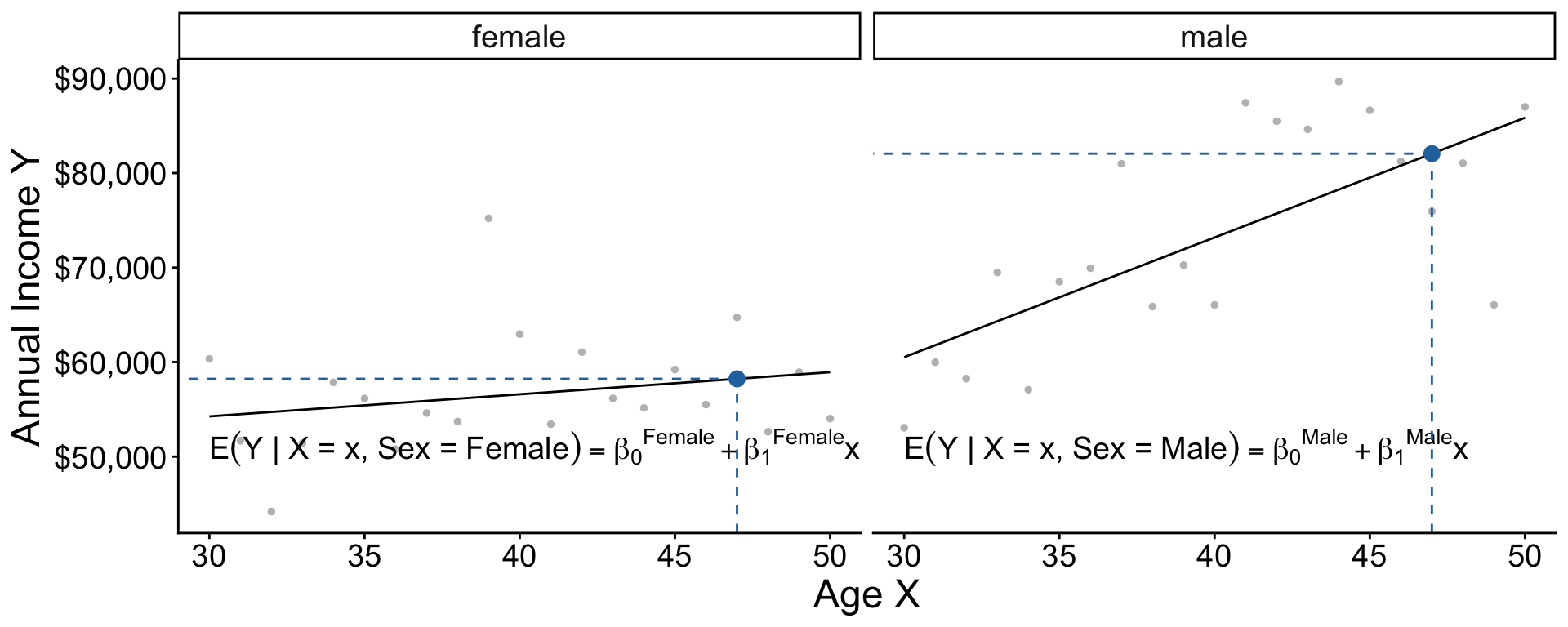
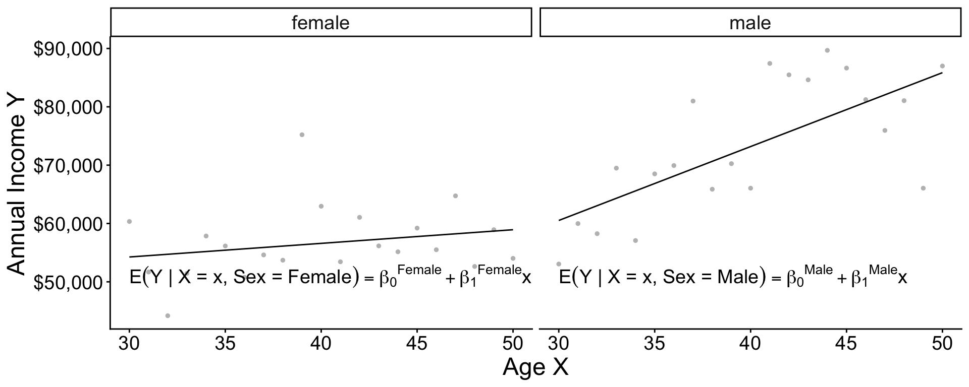
Two models: Interaction

\[ \begin{aligned} \text{E}(Y\mid X, \text{Female}) &= \beta_0^\text{Female} + \beta_1^\text{Female}\times \text{Age} \\ \text{E}(Y\mid X, \text{Male}) &= \beta_0^\text{Male} + \beta_1^\text{Male}\times \text{Age} \\ \end{aligned} \]

Equivalently, \[\text{E}(Y \mid X, \text{Sex}) = \gamma_0 + \gamma_1(\text{Female}) + \gamma_2(\text{Age}) + \gamma_3 (\text{Age} \times \text{Female})\] . . .

where \[\begin{aligned} \gamma_0 &= \beta_0^\text{Male} &\gamma_1 &= \beta_0^\text{Female} - \beta_0^\text{Male} \\ \gamma_2 &= \beta_1^\text{Male} &\gamma_3 &= \beta_1^\text{Female} - \beta_1^\text{Male} \end{aligned}\]

Two models: Interaction in code

Generate data in 2019 that vary in both sex and age

all_2019 <- simulated |>
  filter(year == 2019)

# A tibble: 3,204 × 4
   year   age sex   income
  <dbl> <dbl> <chr>  <dbl>
1  2019    41 male  50285.
2  2019    45 male  31057.
3  2019    34 male  66166.
# ℹ 3,201 more rows

Two models: Interaction in code

The * operator allows slopes to differ across groups

model <- lm(
  formula = income ~ sex * age,
  data = all_2019
)

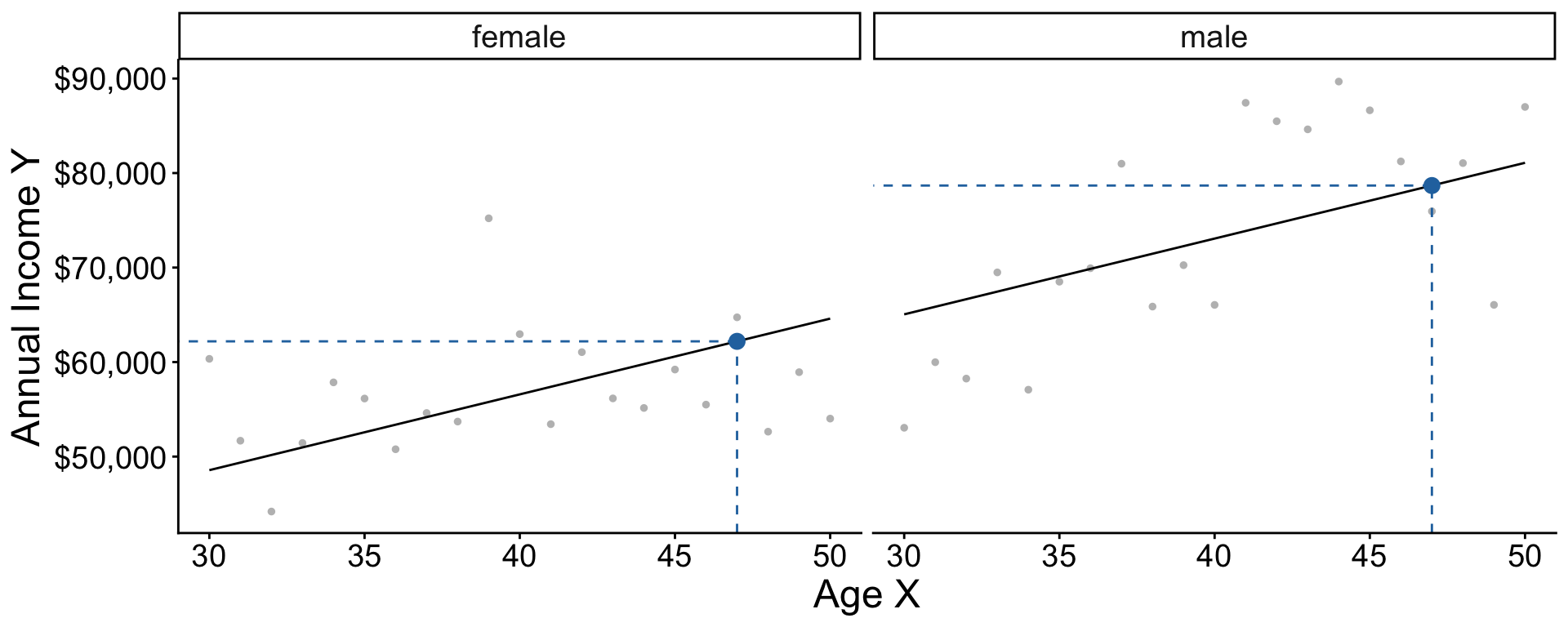
Two models: Additive model in R

The + operator assumes slopes are the same across groups

model <- lm(
  formula = income ~ sex + age,
  data = all_2019
)

Interactions make lots of terms

model <- lm(
  formula = income ~ sex * age * year,
  data = simulated
)

summary(model)


Call:
lm(formula = income ~ sex * age * year, data = simulated)

Residuals:
   Min     1Q Median     3Q    Max 
-81158 -33849 -14946  15839 972817 

Coefficients:
                   Estimate Std. Error t value Pr(>|t|)
(Intercept)       1.387e+06  2.343e+06   0.592    0.554
sexmale          -1.943e+06  3.117e+06  -0.623    0.533
age              -6.273e+04  5.760e+04  -1.089    0.276
year             -6.680e+02  1.163e+03  -0.574    0.566
sexmale:age       6.646e+04  7.675e+04   0.866    0.386
sexmale:year      9.519e+02  1.547e+03   0.615    0.538
age:year          3.130e+01  2.859e+01   1.095    0.274
sexmale:age:year -3.247e+01  3.809e+01  -0.852    0.394

Residual standard error: 57790 on 29992 degrees of freedom
Multiple R-squared:  0.03332,   Adjusted R-squared:  0.03309 
F-statistic: 147.7 on 7 and 29992 DF,  p-value: < 2.2e-16

Interactions make lots of terms

Penalized Regression

Penalized regression

OLS is a linear model

\[\text{E}(Y\mid\vec{X}) = \beta_0 + \beta_1 X_1 + \beta_2 X_2 + \cdots\]

There are many linear models beyond OLS.

(other ways of estimating the \(\beta\) coefficients)

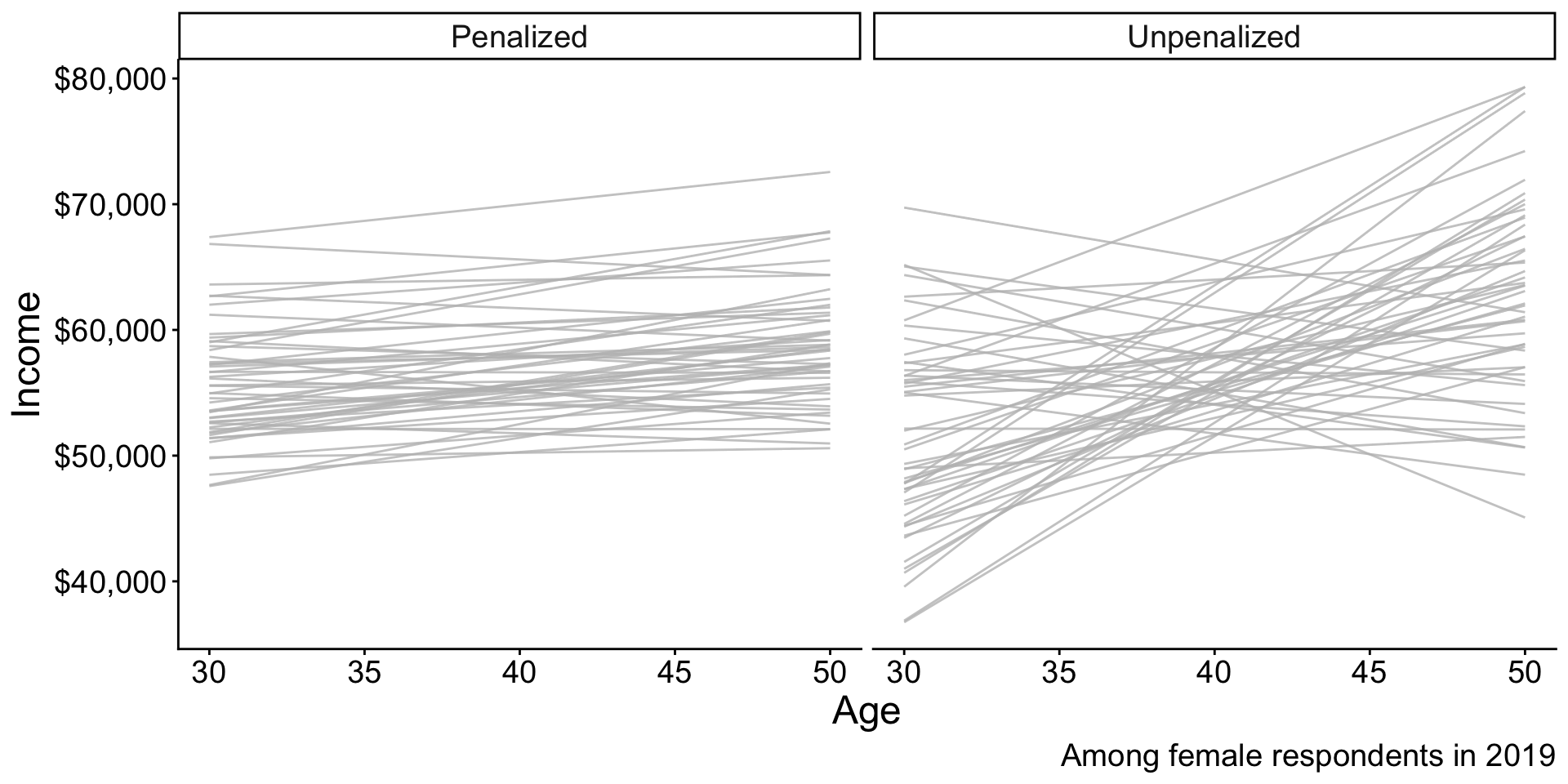
Penalized regression

Unpenalized regression: In math

OLS chose \(\alpha, \vec\beta\) to minimize this function: \[ \begin{aligned} \underbrace{\sum_i\left(Y_i - \hat{Y}_i\right)^2}_\text{Sum of Squared Error} \end{aligned} \] where \(\hat{Y}_i = \hat\alpha + \sum_j X_j \hat\beta_j\)

Penalized regression: In math

Penalized (ridge) regression chose \(\alpha, \vec\beta\) to minimize this function: \[ \begin{aligned} \underbrace{\sum_i\left(Y_i - \hat{Y}_i\right)^2}_\text{Sum of Squared Error} + \underbrace{\lambda \sum_{j} \beta_j^2}_\text{Penalty Term} \end{aligned} \] where \(\hat{Y}_i = \hat\alpha + \sum_j X_j \hat\beta_j\)

Penalized regression: Code

simulated <- simulate(n = 1e5)

Penalized regression: Code

The glmnet package supports penalized regression

library(glmnet)

Penalized regression: Code

Create a model matrix of predictors

Each column will correspond to a coefficient

X <- model.matrix(~ age * sex * year, data = simulated)

Create a vector of the outcomes

y <- simulated |> pull(income)

Penalized regression: Code

Use the cv.glmnet function

penalized <- cv.glmnet(
  x = X,    # model matrix we created
  y = y,    # outcome vector we created
  alpha = 0 # penalize sum of beta ^ 2
)

Penalized regression: Code

yhat <- predict(
  penalized,
  newx = X
)

summary(yhat)

   lambda.1se   
 Min.   :60582  
 1st Qu.:62568  
 Median :65476  
 Mean   :65063  
 3rd Qu.:67425  
 Max.   :69405

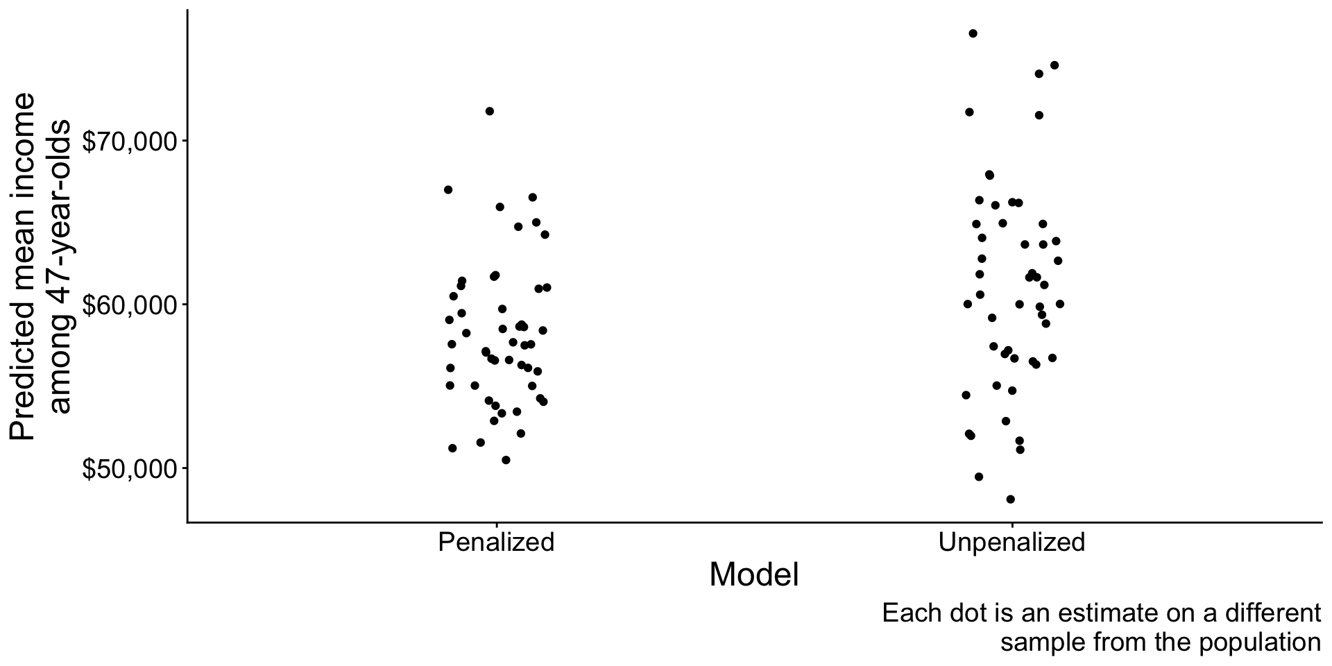
When to use penalized regression?

Many predictors and few observations
- High-variance estimates

When you are willing to accept bias
- Model will be a bit wrong on average