Logistic Regression

UCLA Soc 114

Logistic regression: Learning goals

Some things you may know

• Logistic regression is good for binary outcomes
• Coefficients are hard to interpret

Data science ideas

• Predicted values make logistic regression easy to use

Logistic regression

• A type of model for a binary outcome
  • \(Y\) taking the values {0,1} or {FALSE,TRUE}
• Modeled as a function of predictor variables \(\vec{X}\)

A data example

baseball_population.csv

population <- read_csv("https://soc114.github.io/data/baseball_population.csv")

# A tibble: 944 × 6
  player               salary position team    team_past_record team_past_salary
  <chr>                 <dbl> <chr>    <chr>              <dbl>            <dbl>
1 Bumgarner, Madison 21882892 LHP      Arizona            0.457         2794887.
2 Marte, Ketel       11600000 2B       Arizona            0.457         2794887.
3 Ahmed, Nick        10375000 SS       Arizona            0.457         2794887.
4 Kelly, Merrill      8500000 RHP      Arizona            0.457         2794887.
5 Walker, Christian   6500000 1B       Arizona            0.457         2794887.
# ℹ 939 more rows

A data example

• player is the player name
• salary is the 2023 salary
• position is the position played (e.g., LHP for left-handed pitcher)
• team is the team name
• team_past_record was the team’s win percentage in the previous season
• team_past_salary was the team’s average salary in the previous season

A binary outcome

• You see a player’s salary
• Are they a catcher?
  • position == "C"

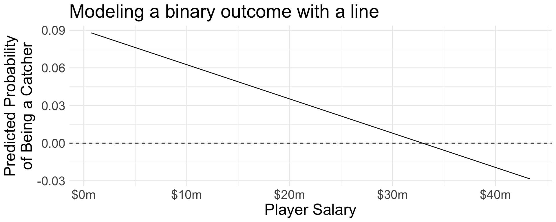
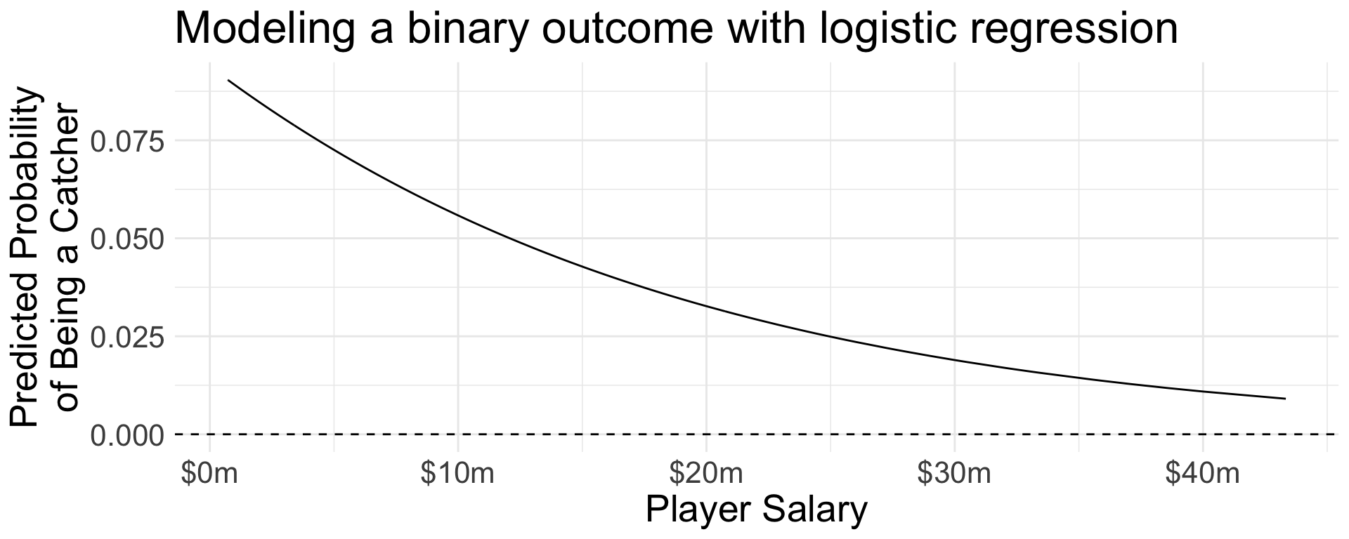
Linear probability model

We can model with lm() for a linear fit.

ols_binary_outcome <- lm(
  position == "C" ~ salary,
  data = population
)

population |>
  mutate(yhat = predict(ols_binary_outcome)) |>
  ggplot(aes(x = salary, y = yhat)) +
  geom_line() +
  geom_hline(yintercept = 0, linetype = "dashed") +
  scale_x_continuous(
    name = "Player Salary",
    labels = label_currency(scale = 1e-6, suffix = "m")
  ) +
  scale_y_continuous(
    name = "Predicted Probability\nof Being a Catcher"
  ) +
  ggtitle("Modeling a binary outcome with a line")

Goal: Avoid illogical predictions

In OLS, there is a linear predictor \[ \mu = \beta_0 + X_1\beta_1 + X_2\beta_2 + \cdots \] that can take any numeric value. Possibly \(\mu <0\) or \(\mu > 1\).

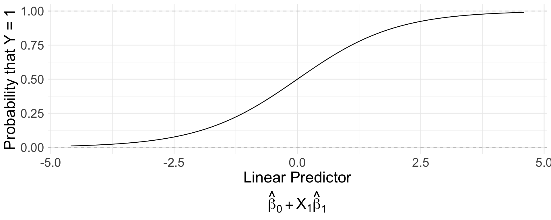
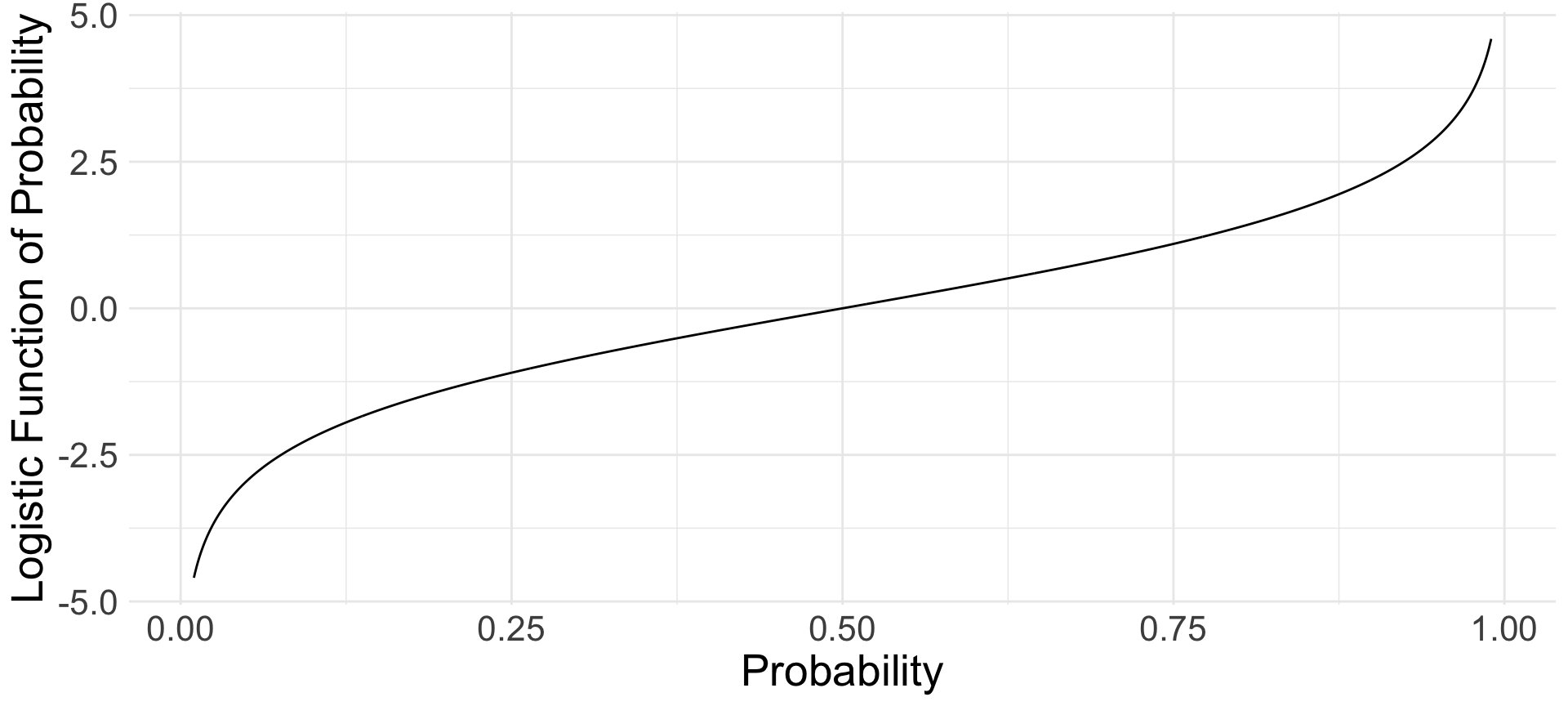
From \(\mu\) to \(\pi\)

Logistic regression passes the linear predictor \[\mu = \beta_0 + X_1\beta_1 + X_2\beta_2 + \cdots\] through a nonlinear function to force it between 0 and 1.

\[ \pi = \text{logit}^{-1}\left(\beta_0 + X\beta_1\right) = \frac{e^{\beta_0 + X\beta_1}}{1 + e^{\beta_0 + X\beta_1}} \]

From \(\mu\) to \(\pi\)

• At linear predictor 0, what is the predicted probability?
• At linear predictor 2.5, what is the predicted probability?
• At linear predictor \(\infty\), what is the predicted probability?

From \(\pi\) to \(\mu\)

You can also think from \(\pi\) to \(\mu\).

\[ \begin{aligned} \text{logit}(\pi) &= \mu = \beta_0 + X\beta_1 \\ \log\left(\frac{\pi}{1-\pi}\right) &= \mu = \beta_0 + X\beta_1 \end{aligned} \]

From \(\pi\) to \(\mu\)

Logistic regression in R

The glm() function (for logistic regression) works exactly like the lm() function (for linear regression)

Logistic regression in R

logistic_regression <- glm(
  position == "C" ~ salary,
  data = population,
  family = "binomial"
)

• position == "C" is our outcome: the binary indicator that the position variable takes the value "C"
• salary is a predictor variable
• family = "binomial" specifies logistic regression (since “binomial” is a distribution for binary outcomes)

Coefficients: A word of warning

Hard to interpret. Not probabilities. Use predicted values instead.

summary(logistic_regression)

Call:
glm(formula = position == "C" ~ salary, family = "binomial", 
    data = population)

Coefficients:
              Estimate Std. Error z value Pr(>|z|)    
(Intercept) -2.268e+00  1.500e-01 -15.126   <2e-16 ***
salary      -5.599e-08  2.599e-08  -2.154   0.0312 *  
---
Signif. codes:  0 '***' 0.001 '**' 0.01 '*' 0.05 '.' 0.1 ' ' 1

(Dispersion parameter for binomial family taken to be 1)

    Null deviance: 508.94  on 943  degrees of freedom
Residual deviance: 502.85  on 942  degrees of freedom
AIC: 506.85

Number of Fisher Scoring iterations: 6

Predicted values

Be sure to use type = "response" predict probabilities (between 0 and 1) instead of log odds

predict(
  logistic_regression,
  type = "response"
)

Predicted values

population |>
  mutate(yhat = predict(logistic_regression, type = "response")) |>
  distinct(salary, yhat) |>
  ggplot(aes(x = salary, y = yhat)) +
  geom_line() +
  geom_hline(yintercept = 0, linetype = "dashed") +
  scale_x_continuous(
    name = "Player Salary",
    labels = label_currency(scale = 1e-6, suffix = "m")
  ) +
  scale_y_continuous(
    name = "Predicted Probability\nof Being a Catcher"
  ) +
  ggtitle("Modeling a binary outcome with logistic regression")

Predicted values with newdata

• New player: salary is $5 million.
• What is the probability that this player is a catcher?

to_predict <- tibble(salary = 5e6)

Make the predicted value.

predict(
  logistic_regression,
  newdata = to_predict,
  type = "response"
)

         1 
0.07255671 

Linear and logistic regression

What is the same? What is different?

• Same
  • Takes \(X\) and predicts \(Y\)
  • Involves \(\beta_0 + \beta_1 X\)
• Different
  • Logistic regression predicts a probability \(0\leq\pi\leq 1\)

\[ \log\left(\frac{\pi}{1-\pi}\right) = \beta_0 + X_1\beta_1 \]

Logistic regression: Learning goals

Some things you may know

• Logistic regression is good for binary outcomes
• Coefficients are hard to interpret

Data science ideas

• Predicted values make logistic regression easy to use