Mean Squared Error: In and Out of Sample
Use data to learn a model. What does that mean?
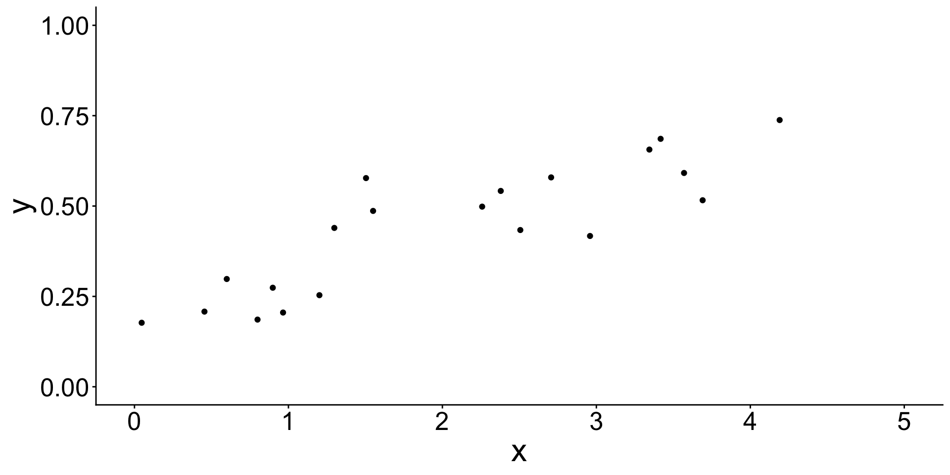
Begin with some data. Assume a linear model.
![]()
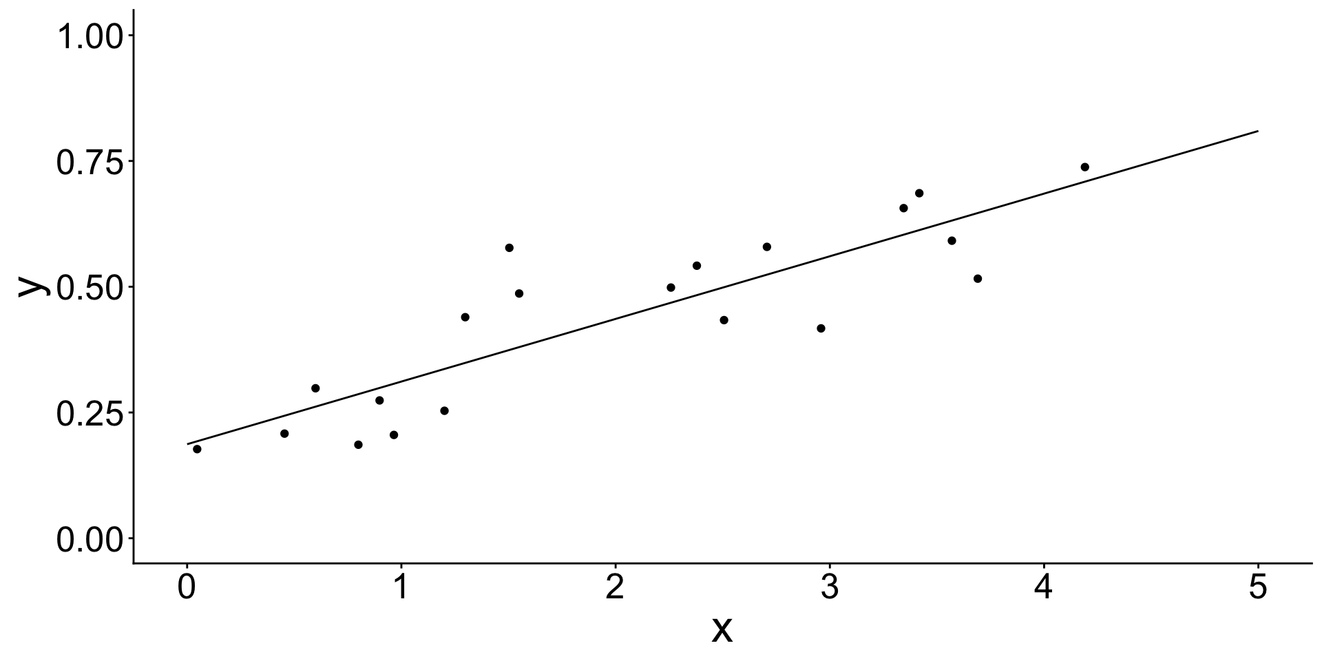
Estimate a linear model
Call:
lm(formula = y ~ x, data = simulated)

Residuals:
      Min        1Q    Median        3Q       Max
-0.138289 -0.069877  0.006674  0.056056  0.203069

Coefficients:
            Estimate Std. Error t value Pr(>|t|)
(Intercept)  0.18696    0.03969    4.71 0.000175 ***
x            0.12455    0.01688    7.38 7.58e-07 ***
---
Signif. codes:  0 '***' 0.001 '**' 0.01 '*' 0.05 '.' 0.1 ' ' 1

Residual standard error: 0.09133 on 18 degrees of freedom
Multiple R-squared:  0.7516,    Adjusted R-squared:  0.7378
F-statistic: 54.47 on 1 and 18 DF,  p-value: 7.578e-07
Estimate a linear model
![]()
The model learned coefficient values from the data.
![]()
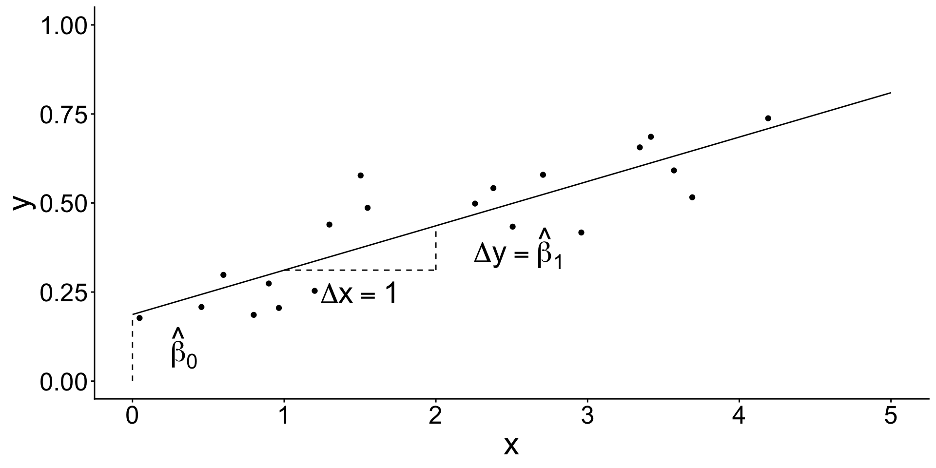
How? It learned by minimizing the sum of squared errors
![]()
How? It learned by minimizing the sum of squared errors
\[
\begin{aligned}
\text{Sum of squared error:}\qquad &\sum_{i\in\text{learning}} \left(y_i - \hat{y}_i\right) ^ 2 \\
\text{Mean squared error:}\qquad &\frac{1}{n_\text{Learning}}\sum_{i\in\text{learning}} \left(y_i - \hat{y}_i\right)
\end{aligned}
\]
- We estimated the line in
learning data
- Now we evaluate the estimated line in
testing data
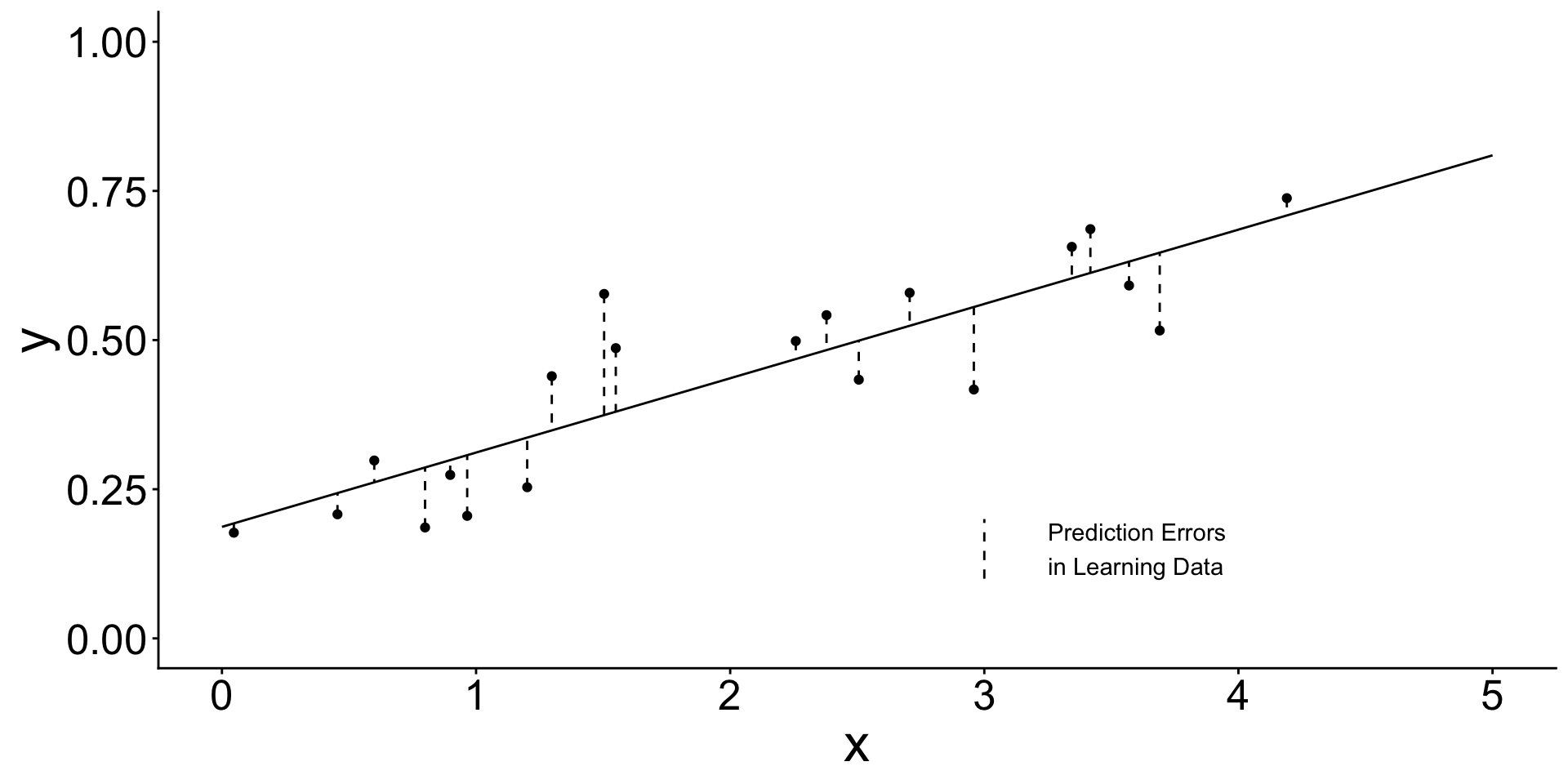
Learning data (used to estimate the line)
![]()
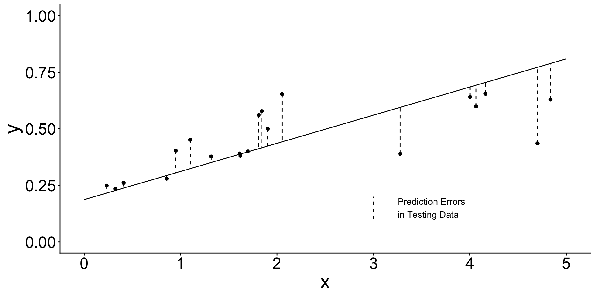
Testing data (used to evaluate the already-learned line)
![]()
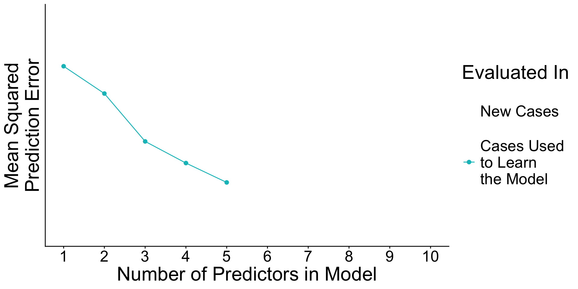
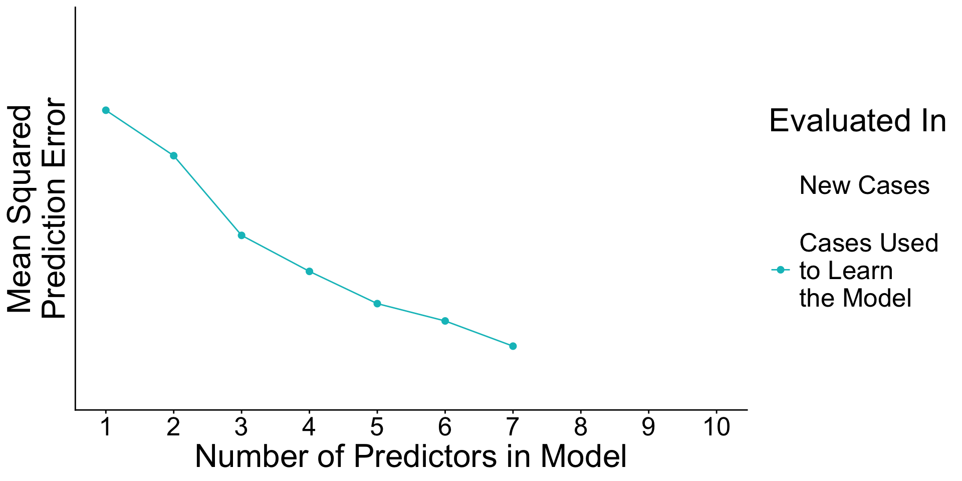
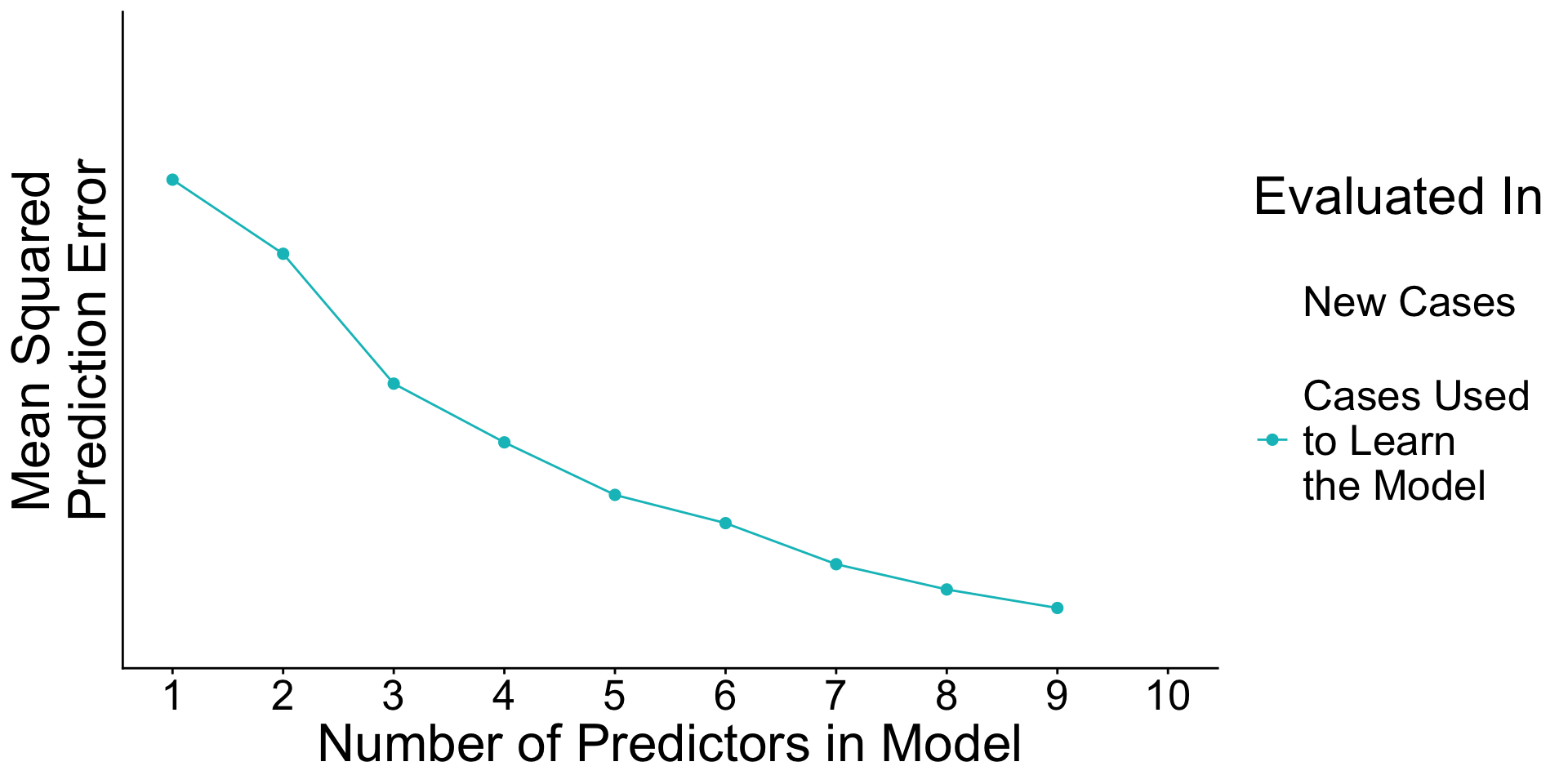
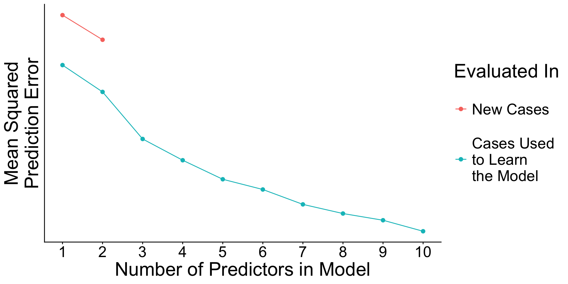
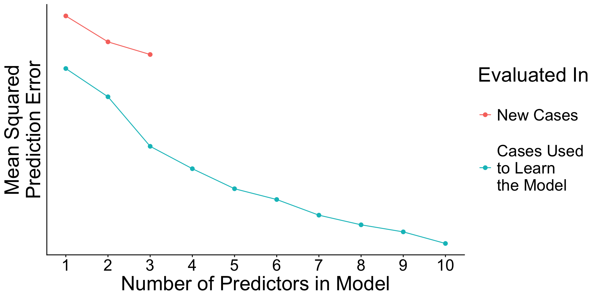
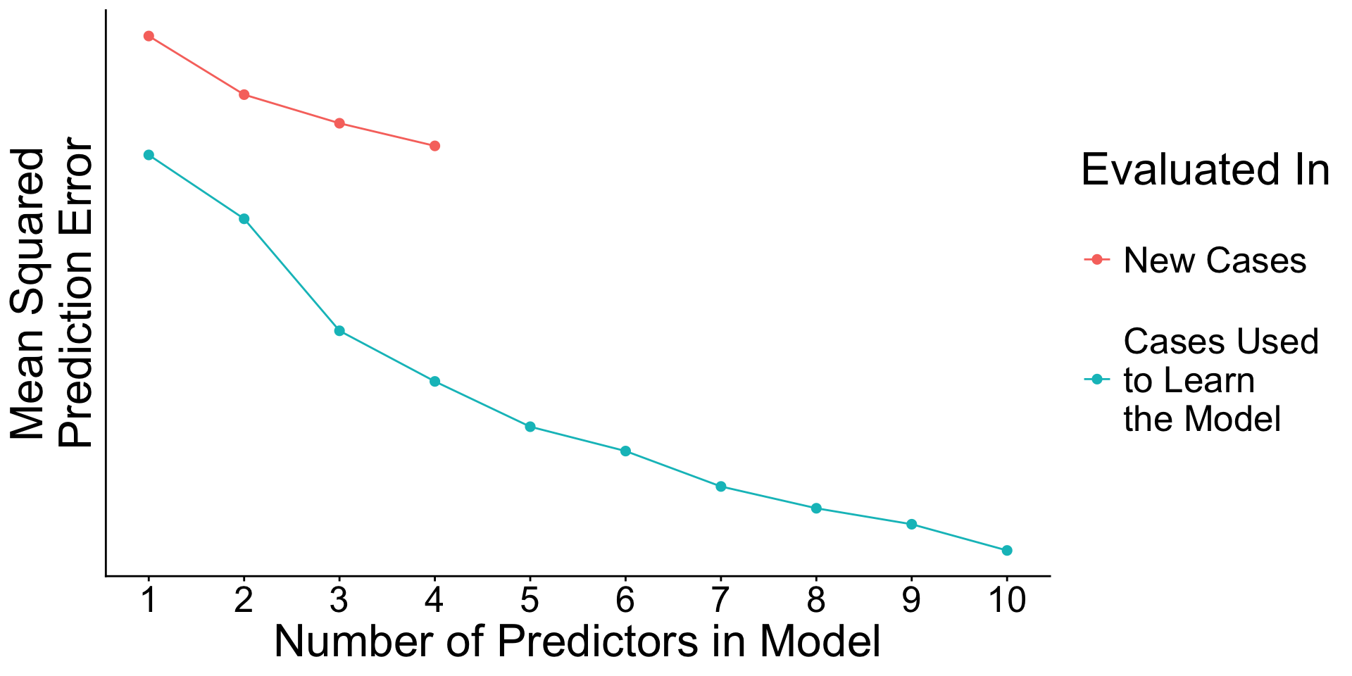
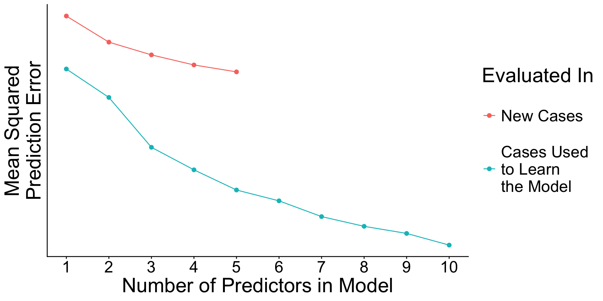
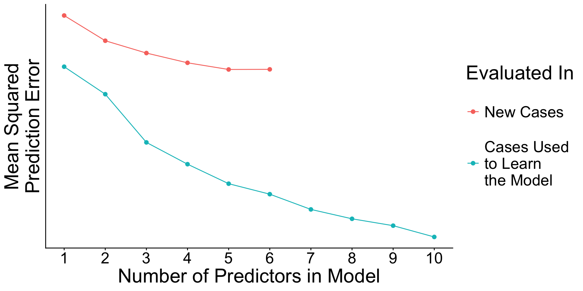
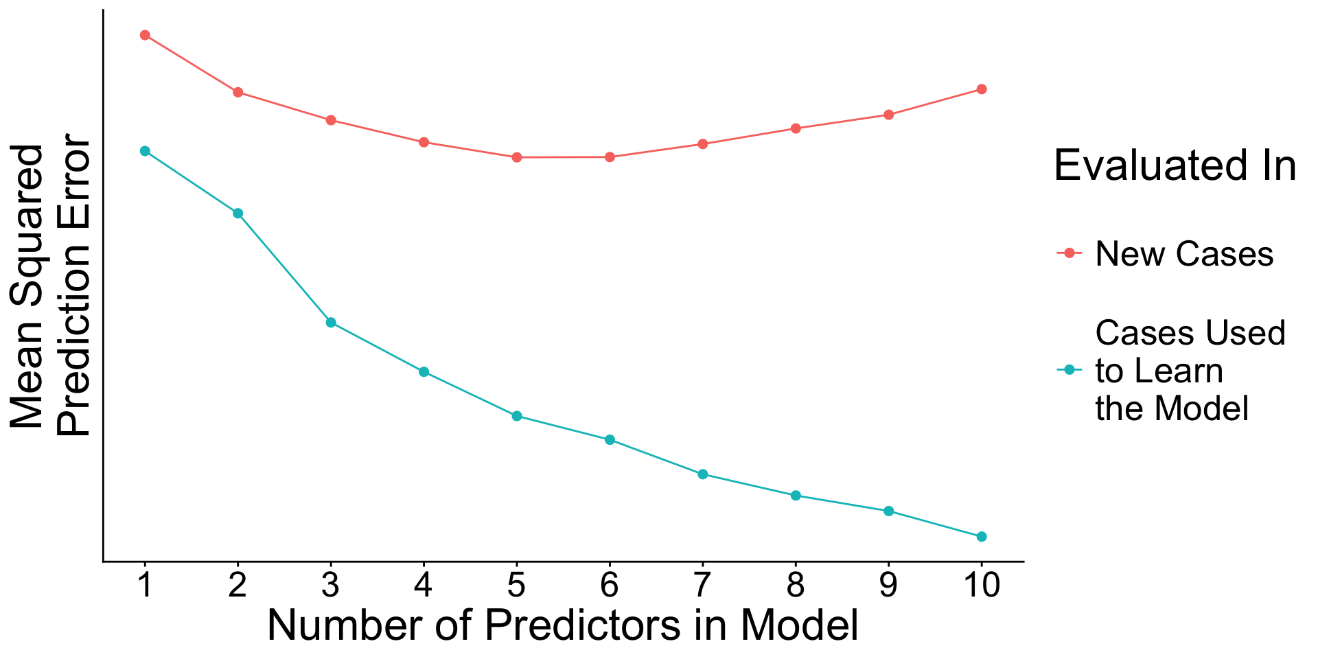
When will prediction errors in learning and testing data differ?
True model:
\[
\text{E}\left(Y\mid\vec{X}\right) = X_1\beta_1 + X_2\beta_2 + ... + X_{10}\beta_{10}
\] with \(\beta_1 = .9\), \(\beta_2 = 0.8\), , \(\beta_9 = 0.1\), \(\beta_{10} = 0\).
We observe \(n = 300\) cases.
Recap: Surprising facts
- An estimated model picks up both
- Signal. True patterns linking \(\vec{X}\) to \(Y\)
- Noise. Random patterns particular to the learning data.
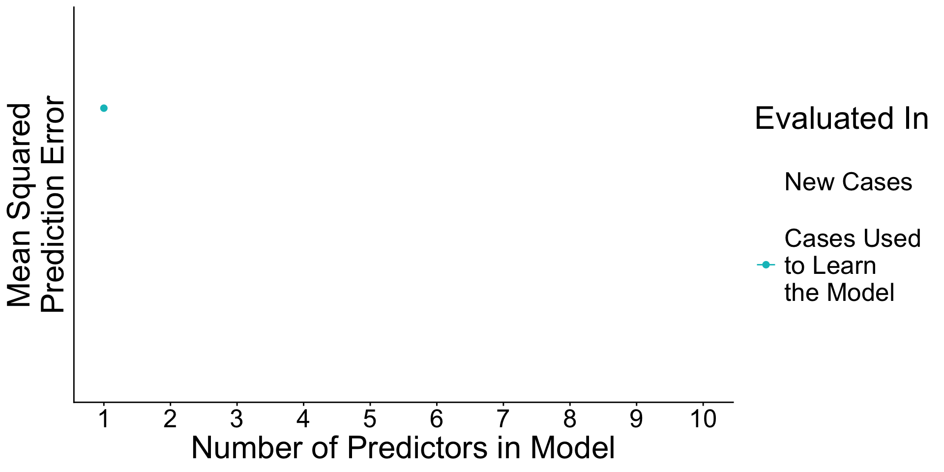
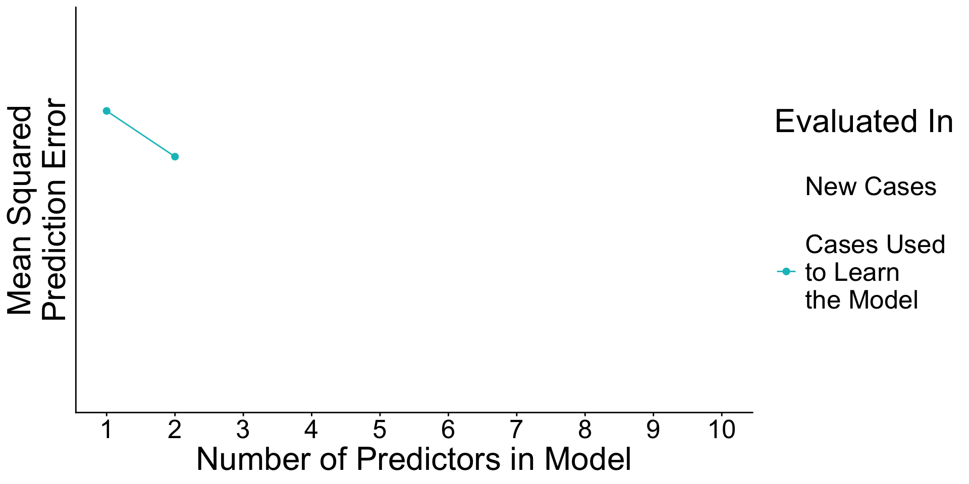
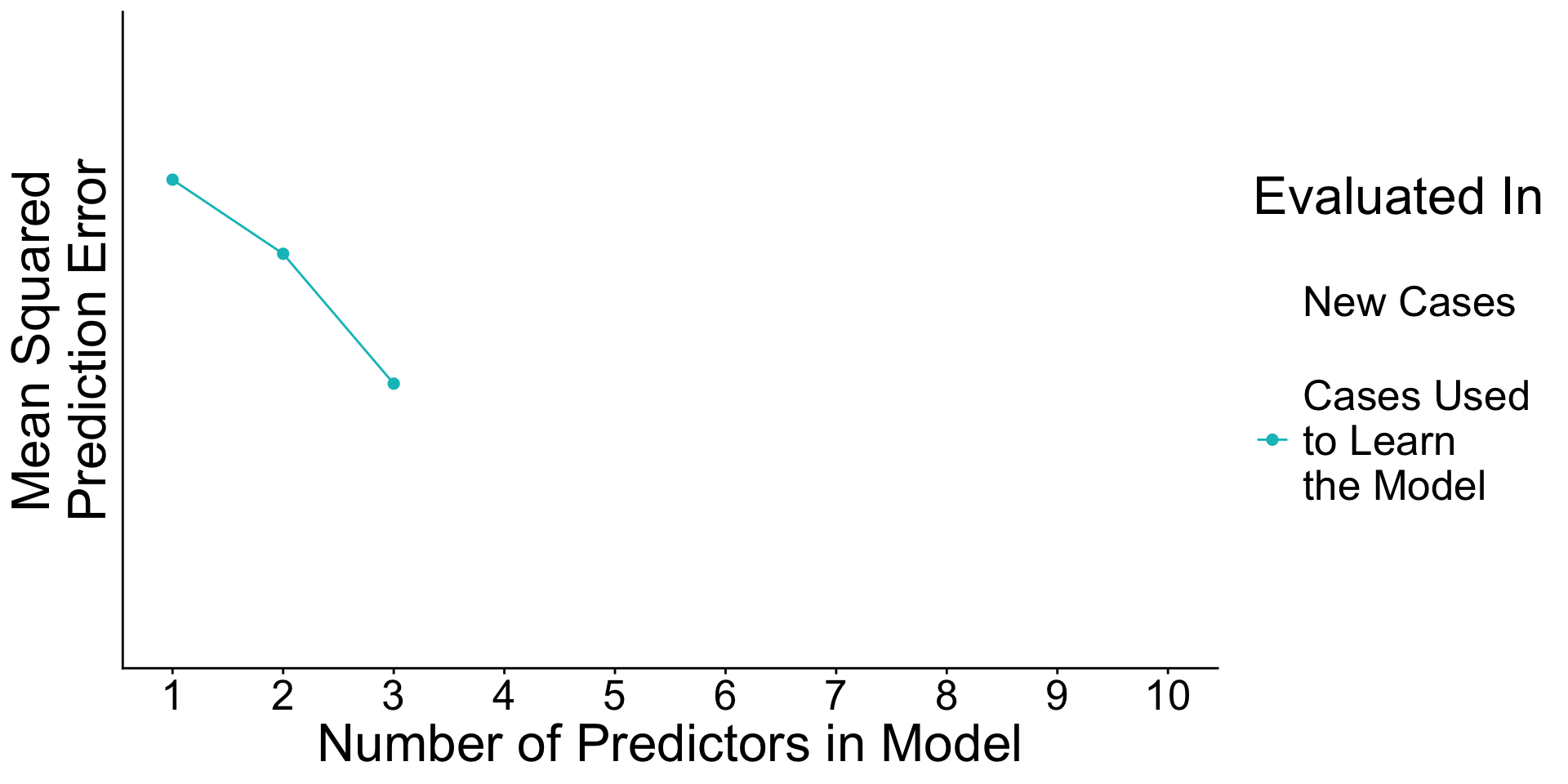
Recap: Surprising facts
- As you add predictors to the model
- error in learning data goes down
- error in testing data may go up
Why? With many predictors, the noise may dominate the signal.
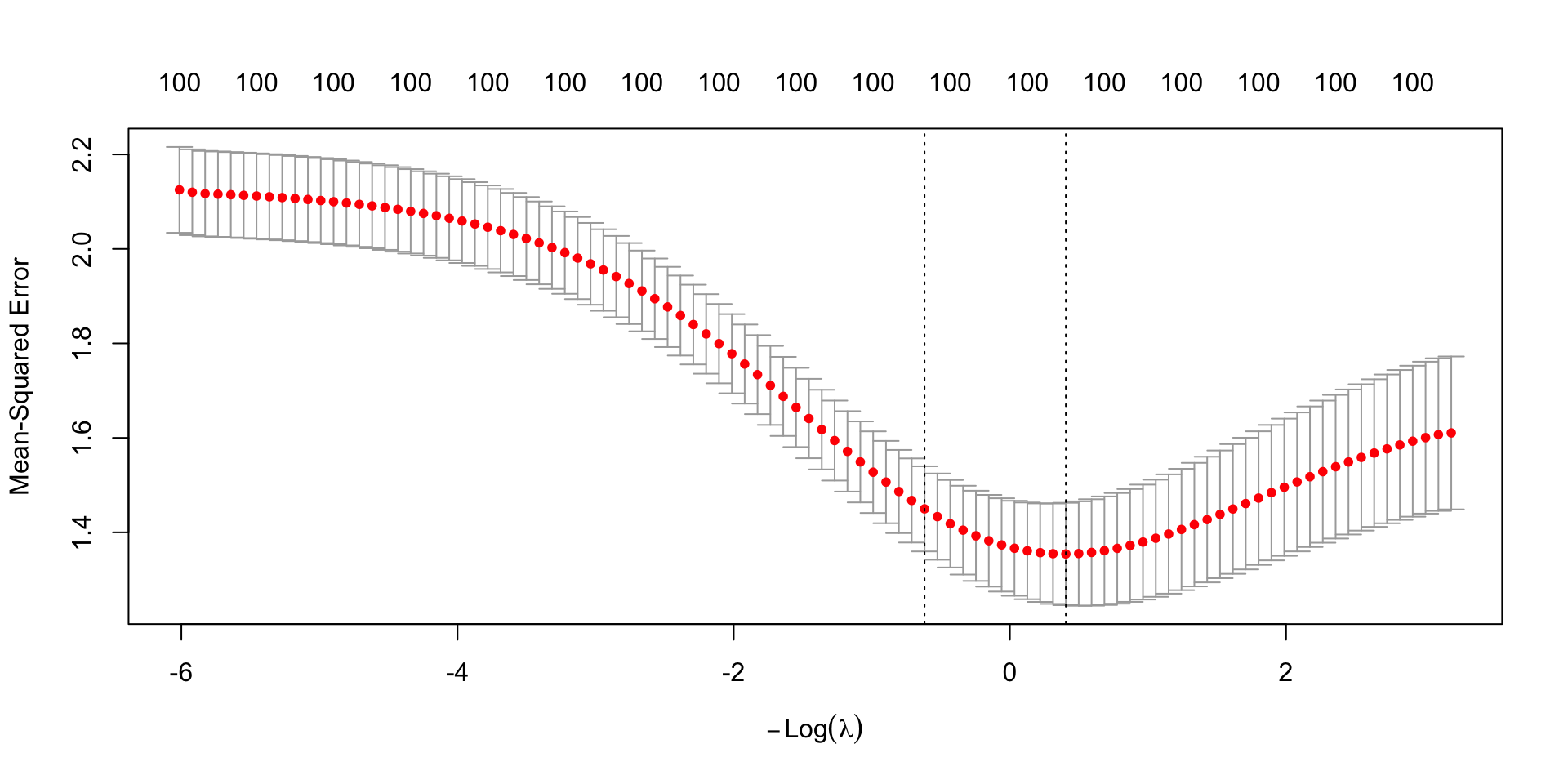
A use case for train and test: Tuning parameters
for_sample_split <- read_csv("https://soc114.github.io/assets/for_sample_split.csv")
- Predictors
x1 through x100
- Outcome
y
- \(n\) = 300 cases
A use case for train and test: Tuning parameters
Recall penalized (ridge) regression. Chooses \(\vec\beta\) to minimize
\[
\begin{aligned}
\underbrace{\sum_i\left(Y_i - \hat{Y}_i\right)^2}_\text{Sum of Squared Error} + \underbrace{\lambda \sum_{j} \beta_j^2}_\text{Penalty Term}
\end{aligned}
\]
But how to choose \(\lambda\)?
A use case for train and test: Tuning parameters
library(glmnet)
X <- model.matrix(y ~ ., data = for_sample_split)
y <- for_sample_split |> pull(y)
penalized_regression <- cv.glmnet(x = X, y = y, alpha = 0)
cv.glmnet chooses \(\lambda\) for you. How?
A use case for train and test: Tuning parameters
plot(penalized_regression)
![]()
It chooses \(\lambda\) to minimize out-of-sample prediction error.
Recap: Data-driven model selection
When there are many candidate models, you can choose the one with the lowest out-of-sample mean squared error.