parents <- read_csv("https://soc114.github.io/data/parents.csv")Problem Set 4: Statistical Learning
Gender inequality in employment is much greater among new parents than among non-parents. This exercise seeks to estimate the proportion employed among married men and women1 with a 1-year-old child at home. Our data include those with at least one child age 0–18.
Synthetic data
To speed data access, we downloaded data from the basic monthly Current Population Survey for all months from 2010–2019. We processed these data, grouped by sex and age of the youngest child, and estimated the proportion employed. We then generated synthetic data: we created a new dataset for you to use with simulated people using these known probabilities.
Synthetic data is good in our setting for two reasons
- we know the answer
- you can download the synthetic data right from this website
For transparency, here is the code with which we created the synthetic data. The line below will load the synthetic data.
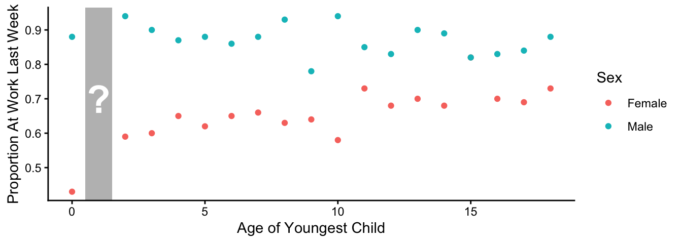
Your synthetic data intentionally omits any parents with child age 1. Here is a graph showing the averages in your data, grouped by child age and sex.
Your task
Predict the proportion employed among female respondents whose youngest child is 1 year old.
This subgroup at which to make a prediction is:
target_population <- tibble(sex = "female", child_age = 1)You will estimate several models to predict at_work as a function of sex and child_age.
Linear regression
- Estimate an additive OLS model for
at_workas an additive function ofsexandchild_age. Store it inols_additive. - Visualize the additive model. Create a
ggplot()in which the \(x\)-axis ischild_age, the color issex, and the \(y\)-axis has predictions fromols_additive. Store this plot inols_additive_plot. - Estimate an interactive OLS model for
at_workas a interactive function ofsexandchild_age. Store it in an objectols_interactive. - Visualize the interactive model. Create a
ggplot()in which the \(x\)-axis ischild_age, the color issex, and the \(y\)-axis has predictions fromols_interactive. Store this plot inols_interactive_plot. - Use either OLS model to predict the outcome in the target population. Store your predicted value (a number) in an object
ols_prediction.
Logistic regression
- Estimate a logistic regression model to predict
at_workas a function ofsexandchild_age. You can use any functional form you want. Store it in an objectlogistic_regression. - Visualize the logistic regression model. Create a
ggplot()in which the \(x\)-axis ischild_age, the color issex, and the \(y\)-axis has predictions fromlogistic_regression. Store this plot inlogistic_plot. - Use your logistic regression model to predict the probability of being
at_workin the target population. Store your predicted value (a number) in an objectlogistic_prediction.
Your approach
Ultimately, this problem set is a challenge: who can best predict the outcome in target_population?
You can use any approach. A model from above, one of them learned on data from a subgroup (e.g., those with child_age under 5), or one with a different functional form (e.g., you can use nonlinear terms for child_age). You can also estimate model-free by taking some subsample mean. You can use any method. If your approach will use a package we have not used in class, let us know on Piazza so that we can ensure the autograder has installed this package.
- Store your predicted probability (a number) for
target_populationin an object calledmy_prediction.
We will extract my_prediction from your submitted problem sets, see who is closest, and announce a winner in class!
Footnotes
Each married pair need not be of different sex. The data include same-sex couples.↩︎