scf_prepared <- read_csv("https://soc114.github.io/data/scf_prepared.csv")Problem Set 3: Estimator and Bootstrap
For this problem set, we will summarize wealth gaps using data from the 2022 Survey of Consumer Finances. We accessed these data via the Berkeley Survey Documentation and Analysis website and prepared the data file scf_prepared.csv that you can load directly with the line of code below.
A row of these data corresponds to a household. These data contain three variables:
raceof the household respondent, coded in categories White, Black, Hispanic, Asian, and Other.wealthis the net worth of the household (assets minus debts), with households below $10,000 recoded to a bottom-code of $10,000weightis a sample weight (the inverse probability of sample inclusion)
Below we have info to get you started. The problem set questions start in the section write an estimator function.
Info to get you started
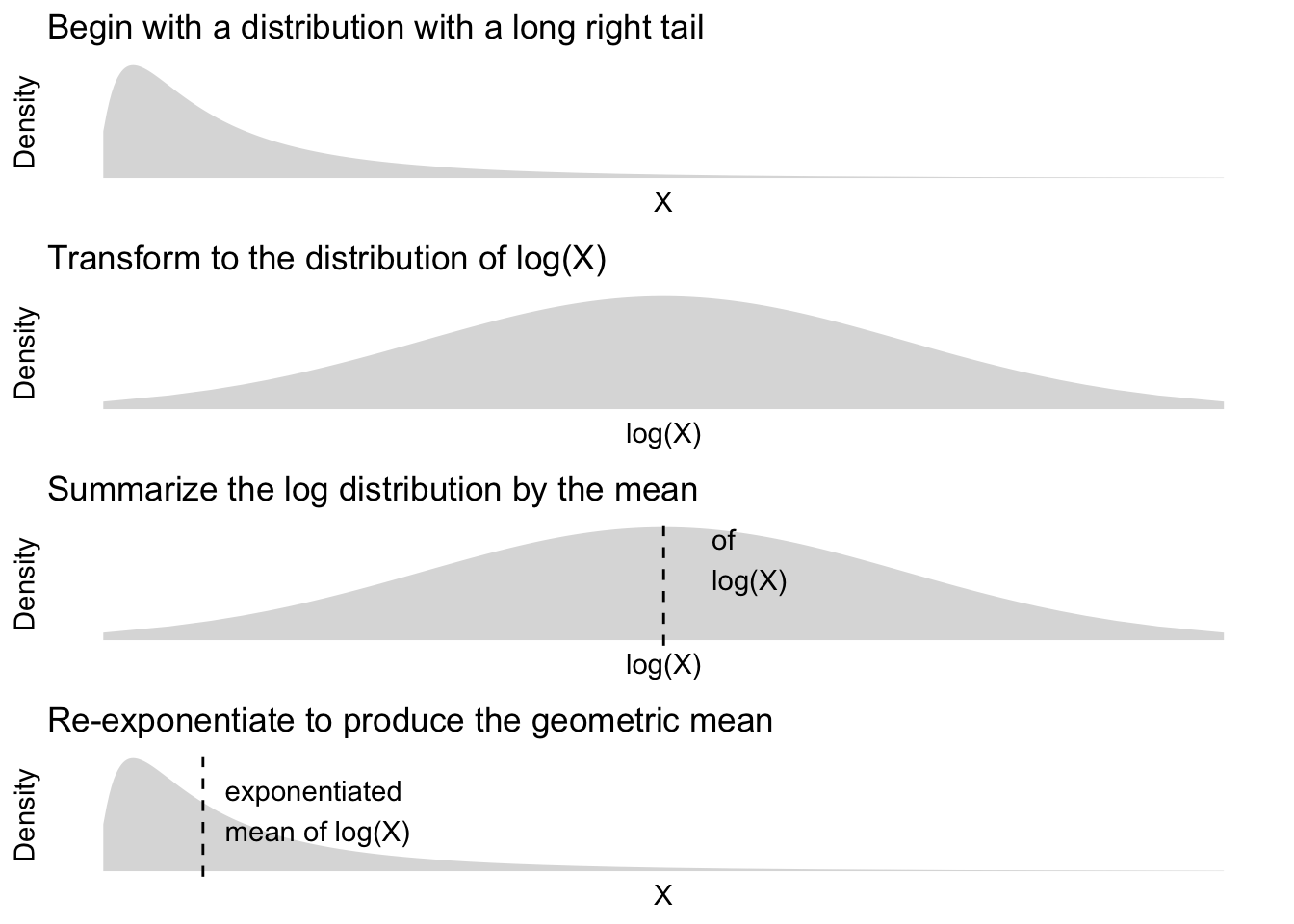
This problem set will summarize wealth by the geometric mean, which is a summary statistic often used for distributions with long right tails. This summary statistic can be understood in steps:
- Transform \(X\) to \(\text{log}(X)\) to bring in the long right tail
- Summarize the transformed distribution by its mean
- Exponentiate the summary to move back to the scale of \(X\) (since \(e^{\text{log}(X)} = X\))
The figure below visualizes these steps to build intuition.
The code below applies these steps to the scf_prepared data to estimate the geometric mean of household wealth.
scf_prepared |>
  # Creates a new variable log_wealth
  # which is the log of the wealth variable
  mutate(
    log_wealth = log(wealth)
  ) |>
  # Summarizes log wealth
  # by its weighted mean
  # (weight is the inverse probability
  # of sample inclusion)
  summarize(
    mean_log_wealth = weighted.mean(
      x = log_wealth,
      w = weight
    )
  ) |>
  # Create a new variable geo_mean which
  # is the exponentiated mean of the log wealth
  mutate(
    geo_mean = exp(mean_log_wealth)
  ) |>
  # Pull the result out of the tibble
  # object to return a number
  pull(geo_mean)
[1] 161195.7Now it is your turn! The code above will be useful in the problem set parts below.
1. Write an estimator function
We want to use the code above many times, on many different samples. To do this, write a function called geo_mean_estimator. Your function should have one argument named data, which will be a tibble object in the format of scf_prepared. Your function should take data and calculate a summary statistic: the geometric mean.
You can use the code above within the body of your function. For help, see R4DS Ch 25.
2. Point estimate
Apply your geo_mean_estimator function with data = scf_prepared. Store the result in an object called geo_mean_estimate.
3. Bootstrap draws
Bootstrap your estimator 1,000 times. Store your bootstrap draws in an object named bootstrap_draws.
How you do this is up to you. There are at least two viable options:
- You can initialize a vector
bootstrap_drawsas in class. Then write a for loop to populate it. See lecture slides on for loops. - You can use the
replicate(n, expr)function where thenargument is the number of times to call the expression in theexprargument. See this blog.
Whatever method you use, you should use slice_sample(prop = 1, replace = TRUE) to resample the dataset with replacement for each bootstrap draw. See lecture slides on how to generate bootstrap samples.
4. Confidence interval
Construct a 95% confidence interval for the geometric mean by taking the 2.5 and 97.5 percentiles of the bootstrap draws. Store this in an object named confidence_interval.
5. Write a ratio estimator
Now write a new function named ratio_estimator that estimates a ratio: \[
\frac{\text{geometric mean among white respondent households}}{\text{geometric mean among Black respondent households}}
\] In words, this summary is how many dollars of wealth White households hold per dollar held by Black households, as summarized by the geometric mean.
You might consider using the geo_mean_estimator() function you already wrote within your ratio_estimator() function.
6. Point estimate for the ratio
Apply ratio_estimator with data = scf_prepared to produce a point estimate. Store the result in ratio_estimate.
7. Bootstrap the ratio estimator
Bootstrap the ratio estimator with 1,000 draws. Store the bootstrap estimates in an object called ratio_bootstrap.
8. Confidence interval for the ratio
Construct a 95% confidence interval for the ratio by taking the 2.5 and 97.5 percentiles of the bootstrap draws. Store this in an object named ratio_confidence_interval.