Difference in Difference

Here are slides

Today we study the effect of a policy change in New Jersey, drawing on evidence from the neighboring state of Pennsylvania.

Difference in difference is an identification strategy to be used when one or more units become treated at some time point while others do not. If we believe an assumption of parallel trends, then we can use the change over time for the never-treated units to estimate the change over time that would have been experienced by the units who become treated, in a counterfactual world where they had not become treated.

Data requirements

To carry out difference in difference, you need

One or more units become treated at an intervention time
- Example: NJ adopts a higher minimum wage
One or more units remain untreated
- Example: PA does not change the minimum wage
Data on all the units before and after the intervention time
- Example: Data on NJ and PA before and after the change

Causal estimand

The causal estimand in DID is typically the average treatment effect on the treated in the post-treatment period. Let \(Y_{it}^a\) be the outcome of unit \(i\) in period \(t\) under treatment value \(a\). The causal estimand is

\[ \tau_\text{ATT} = \frac{1}{\text{Number Treated}}\sum_{i:A_{it}=1}\left(Y_{it}^{1} - Y_{it}^0\right) \]

The fundamental problem of causal inference is that the outcome under control \(Y_{it}^0\) is not observed for unit \(i\) who at time \(t\) has become treated. We do not know NJ’s employment rate after the minimum wage policy, which would have persisted if NJ had not adopted a new minimum wage.

The parallel trends assumption

We assume parallel trends: the treated unit would have had the same trend in the outcome over time as the control unit, in the absence of treatment.

In math, this assumption is that the potential outcome under control trends the same in both groups over time,

\[ \text{Parallel Trends Assumption:}\qquad \frac{1}{n_\text{Treated}}\sum_{i:A_{it}=1}\left(Y_{it}^0 - Y_{i,t-1}^0\right) = \frac{1}{n_\text{Untreated}}\sum_{i:A_{it}=0}\left(Y_{it}^0 - Y_{i,t-1}^0\right) \] where \(t\) is the post-intervention time point.

You can’t directly test the parallel trends assumption because \(Y_{it}^0\) is not observed for the treated units in the post-treatment period. But you can assess the credibility of the assumption by examining whether trends are parallel in the pre-treatment period.

In class, we will discuss the credibility of the parallel trends assumption using an empirical example from Malesky, Nguyen, & Tran 2014 as re-analyzed by Egami & Yamauchi 2023.

Worked example: Recentralization in Vietnam

This example uses the malesky2014.csv data from Malesky, Nguyen, & Tran 2014 as re-analyzed by Egami & Yamauchi 2023.

Variables in the data

Variables in the data set:

treatment: binary variable indicating if the record is from the treatment group (\(1\)) or the control group (\(0\))
pro4: educational and cultural program number 4 outcome variable (binary: \(1\) if they participated in the program, \(0\) if not)
tapwater: tap water outcome variable (binary: \(1\) if they drink tap water, \(0\) if not)
agrext: agricultural center outcome variable (binary: \(1\) if they use the center, \(0\) if not)
year: the year the record is from
post_treat: binary variable indicating if the record is from the pre-treatment period (\(0\)) or the post-treatment period (\(0\))

The code below loads the data and selects and renames a few variables we will use.

library(tidyverse)
data <- read_csv("https://soc114.github.io/data/malesky2014.csv") |>
  select(treatment, year, education_culture = pro4) |>
  mutate(
    treatment = factor(treatment, labels = c("Control","Treatment"))
  )

Estimate means within group \(\times\) time

We will first estimate the mean value of the outcome (education_culture) within subgroups defined by treatment and year.

summary_statistics <- data |>
  group_by(treatment, year) |>
  summarize(education_culture = mean(education_culture))

`summarise()` has grouped output by 'treatment'. You can override using the
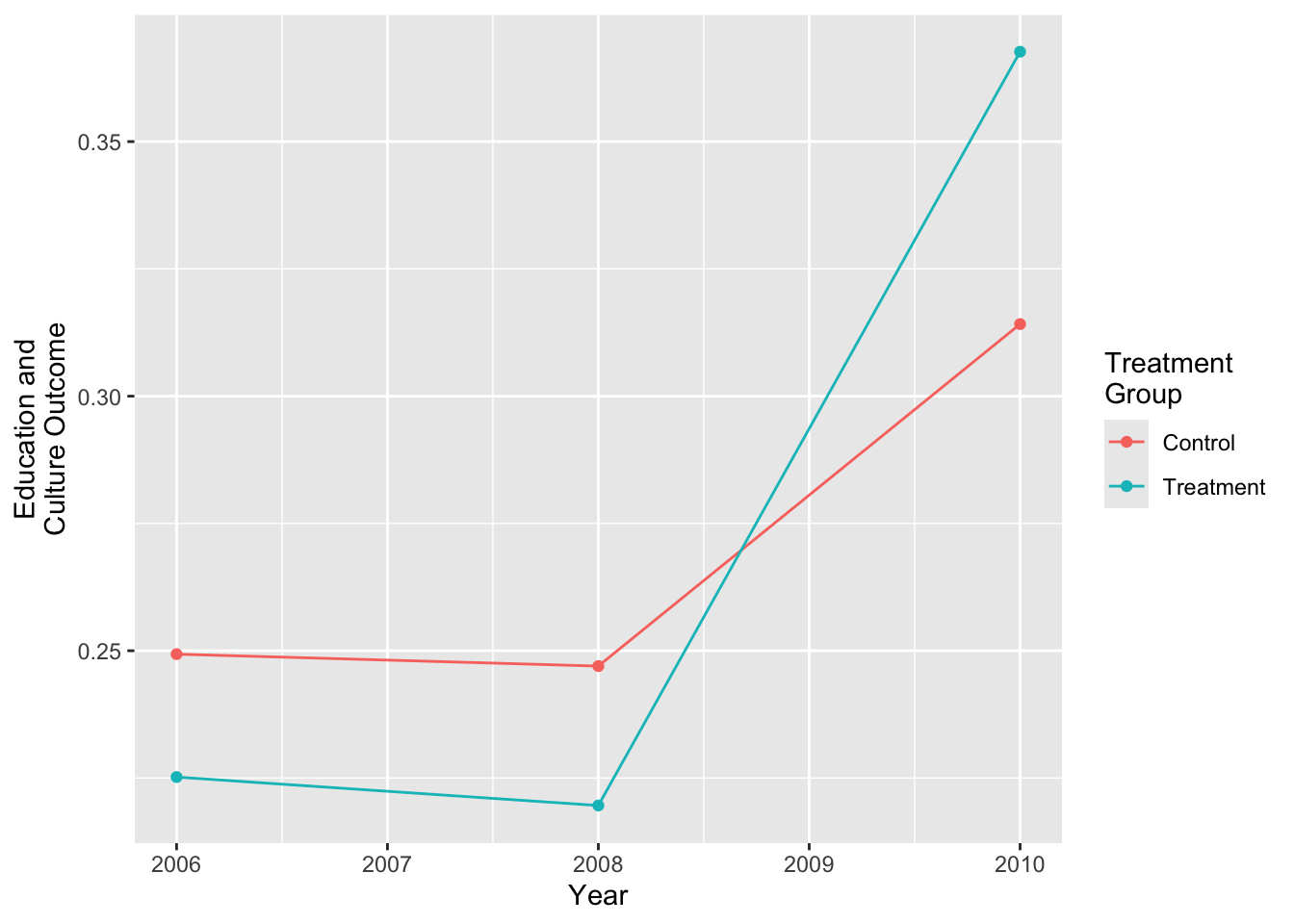
`.groups` argument.

Visualize the trends

We can visualize those summaries using ggplot.

summary_statistics |>
  ggplot(aes(x = year, y = education_culture, color = treatment)) +
  geom_point() +
  geom_line() +
  labs(
    x = "Year",
    y = "Education and\nCulture Outcome",
    color = "Treatment\nGroup"
  )

Produce a difference in difference estimate

We can also estimate the difference in difference.

summary_statistics |>
  pivot_wider(
    names_from = c("treatment","year"), 
    values_from = "education_culture"
  ) |>
  mutate(
    estimate = (Treatment_2010 - Treatment_2008) - 
      (Control_2010 - Control_2008)
  ) |>
  select(estimate)

# A tibble: 1 × 1
  estimate
     <dbl>
1   0.0809