Population sampling

Topic for 1/12.

Claims about inequality are often claims about a population. Our data are typically only a sample! This module addresses the link between samples and populations.

Full count enumeration

What proportion of our class prefers to sit in the front of the room?

We answered this question in class using full count enumeration: list the entire target population and ask them the question. Full count enumeration is ideal because it removes all statistical sources of error. But in settings with a larger target population, the high cost of full count enumeration may be prohibitive.

Simple random sample

We carried out a simple random sample¹ in class.

everyone generated a random number between 0 and 1
those with values less than 0.1 were sampled
our sample estimate was the proportion of those sampled to prefer the front of the room

In a simple random sample, each person in the population is sampled with equal probabilities. Because the probabilities are known, a simple random sample is a probability sample.

Unequal probability sample

Suppose we want to make subgroup estimates:

what proportion prefer the front, among those sitting in the first 3 rows?
what proportion prefer the front, among those sitting in the back 17 rows?

In a simple random sample, we might only get a few or even zero people in the first 3 rows! To reduce the chance of this bad sample, we could draw an unequal probability sample:

those in rows 1–3 are selected with probability 0.5
those in rows 4–20 are selected with probability 0.1

Our unequal probability sample will over-represent the first three rows, thus creating a large enough sample in this subgroup to yield precise estimates.

Having drawn an unequal probability sample, suppose we now want to estimate the class-wide proportion who prefer sitting in the front. We will have a problem: those who prefer the front may be more likely to sit there, and they are also sampled with a higher probability! Sample inclusion is related to the value of our outcome.

Because the sampling probabilities are known, we can correct for this by applying sampling weights, which for each person equals the inverse of the known probability of inclusion for that person.

For those in rows 1–3,

we sampled with probability 50%
on average 1 in every 2 people is sampled
each person in the sample represents 2 people in the population
$w_i = \frac{1}{\text{P}(\text{Sampled}_i)} = \frac{1}{.5} = 2$

For those in rows 4–20,

we sampled with probability 10%
on average 1 in every 10 people is sampled
each person in the sample represents 10 people in the population
$w_i = \frac{1}{\text{P}(\text{Sampled}_i)} = \frac{1}{.1} = 10$

To estimate the population mean, we can use the weighted sample mean,

\[\frac{\sum_i y_iw_i}{\sum_i w_i}\]

Stratified random sample

We could also draw a stratified random sample by first partitioning the population into subgroups (called strata) and then drawing samples within each subgroup. For instance,

sample 10 of the 20 people in rows 1–3
sample 10 of the 130 people in rows 4–17

In simple random or unequal probability sampling, it is always possible that by random chance we sample no one in the front of the room. Stratified random sampling rules this out: we know in advance how our sample will be balanced across the two strata.

Note

In our real-data example at the end of this page, the Current Population Survey is stratified by state so that the Bureau of Labor Statistics knows in advance that they will gather a sufficient sample to estimate unemployment in each state.

A real case: The Current Population Survey

Every month, the Bureau of Labor Statistics in collaboration with the U.S. Census Bureau collects data on unemployment in the Current Population Survey (CPS). The CPS is a probability sample designed to estimate the unemployment rate in the U.S. and in each state.

We will be using the CPS in discussion. This video introduces the CPS and points you toward where you can access the data via IPUMS-CPS.

Example: Baseball players

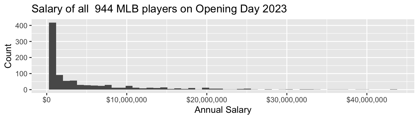
As one example where full-count enumeration is possible, we will examine the salaries of all 944 Major League Baseball Players who were on active rosters, injured lists, and restricted lists on Opening Day 2023. These data were compiled by USA Today and are available in baseball.csv.

baseball <- read_csv("https://soc114.github.io/data/baseball.csv")

# A tibble: 944 × 4
  player            team         position   salary
  <chr>             <chr>        <chr>       <dbl>
1 Scherzer, Max     N.Y. Mets    RHP      43333333
2 Verlander, Justin N.Y. Mets    RHP      43333333
3 Judge, Aaron      N.Y. Yankees OF       40000000
4 Rendon, Anthony   L.A. Angels  3B       38571429
5 Trout, Mike       L.A. Angels  OF       37116667
# ℹ 939 more rows

Salaries are high, and income inequality is also high among baseball players

4% were paid the league minimum of $720,000
53% were paid less than $2,000,000
the highest-paid players—Max Scherzer and Justin Verlander—each earned $43,333,333
the highest-paid half of players take home 92% of the total pay

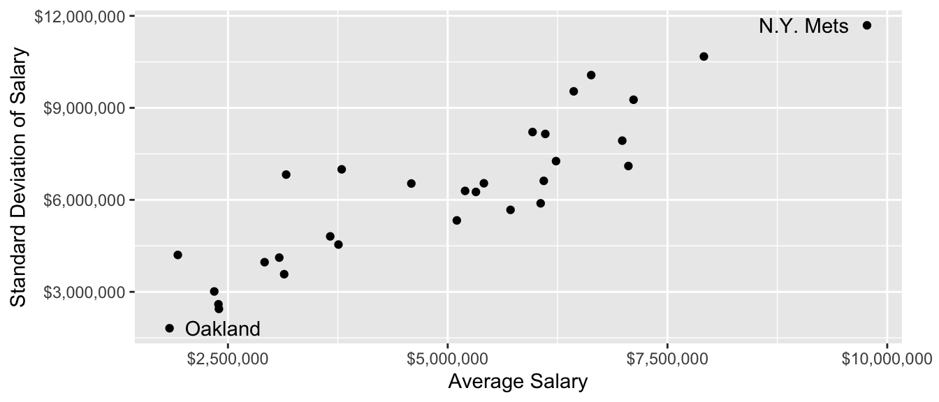
Pay also varies widely across teams!

Conceptualize the sampling strategy

Suppose you did not have the whole population. You still want to learn the population mean salary! How could you learn that in a sample of 60 out of the 944 players?

Before reading on, think through three questions:

What would it mean to use each of these strategies?

a simple random sample of 60 players
a sample stratified by the 30 MLB teams
a sample clustered by the 30 MLB teams

Which strategies have advantages in terms of

being least expensive?
having the best statistical properties?

Given that you already have the population, how would you write some R code to carry out the sampling strategies? You might use sample_n() and possibly group_by().

Sampling strategies in code

In a simple random sample, we draw 60 players from the entire league. Each player’s probability of sample inclusion is $\frac{60}{n}$ where $n$ is the number of players in the league (944).

simple_sample <- function(population) {
  population |>
    # Define sampling probability and weight
    mutate(
      p_sampled = 60 / n(),
      sampling_weight = 1 / p_sampled
    ) |>
    # Sample 60 players
    sample_n(size = 60)
}

To use this function, we give it the baseball data as the population and it returns a tibble containing a sample of 60 players.

simple_sample(population = baseball)

# A tibble: 60 × 6
   player             team         position   salary p_sampled sampling_weight
   <chr>              <chr>        <chr>       <dbl>     <dbl>           <dbl>
 1 Walker, Christian  Arizona      1B        6500000    0.0636            15.7
 2 Fujinami, Shintaro Oakland      RHP       3250000    0.0636            15.7
 3 Tatis, Fernando**  San Diego    OF        7000000    0.0636            15.7
 4 McCann, James*     Baltimore    C        12000000    0.0636            15.7
 5 Merrifield, Whit   Toronto      2B        6750000    0.0636            15.7
 6 Pena, Jeremy       Houston      SS         754900    0.0636            15.7
 7 Harper, Bryce*     Philadelphia OF       27538462    0.0636            15.7
 8 Stubbs, Garrett    Philadelphia C          741000    0.0636            15.7
 9 Mancini, Trey      Chicago Cubs 1B        7000000    0.0636            15.7
10 Walsh, Jared*      L.A. Angels  1B        2650000    0.0636            15.7
# ℹ 50 more rows

In a stratified random sample by team, we sample 2 players on each of 30 teams. A stratified random sample is often a higher-quality sample, because it eliminates the possibility of an unlucky draw that completely omits a few teams. All teams are equally represented no matter what happens in the randomization. The downside of a stratified random sample is that it is costly.

Each player’s probability of sample inclusion is $\frac{2}{n}$ where $n$ is the number on that player’s team (which ranges from 28 to 35).

stratified_sample <- function(population) {
  population |>
    # Draw sample within each team
    group_by(team) |>
    # Define sampling probability and weight
    mutate(
      p_sampled = 2 / n(),
      sampling_weight = 1 / p_sampled
    ) |>
    # Within each team, sample 2 players
    sample_n(size = 2) |>
    ungroup()
}

In a sample clustered by team, we might first sample 3 teams and then sample 20 players on each sampled team. A clustered sample is often less costly, for example because you would only need to call up the front office of 3 teams instead of 30 teams. But this type of sample is lower quality, because there is some chance that one will randomly select a few teams that all have particularly high or low average salaries. A clustered random sample is less expensive but is more susceptible to random error based on the clusters chosen.

Each player’s probability of sample inclusion is P(Team Chosen) $\times$ P(Chosen Within Team) = $\frac{3}{30}\times\frac{20}{n}$ where $n$ is the number on that player’s team (which ranges from 28 to 35).

clustered_sample <- function(population) {
  
  # First, sample 3 teams
  sampled_teams <- population |>
    # Make one row per team
    distinct(team) |>
    # Sample 3 teams
    sample_n(3) |>
    # Store those 3 team names in a vector
    pull()
  
  # Then load data on those teams and sample 20 per team
  population |>
    filter(team %in% sampled_teams) |>
    # Define sampling probability and weight
    group_by(team) |>
    mutate(
      p_sampled = (3 / 30) * (20 / n()),
      sampling_weight = 1 / p_sampled
    ) |>
    # Sample 20 players
    sample_n(20) |>
    ungroup()
}

Weighted mean estimator

Given a sample, how do we estimate the population mean? The weighted mean estimator can also be placed in a function

we hand our sample to the function
we get a numeric estimate back

estimator <- function(sample) {
  sample |>
    summarize(estimate = weighted.mean(
      x = salary, 
      w = sampling_weight
    )) |>
    pull(estimate)
}

Here is what it looks like to use the estimator.

sample_example <- simple_sample(population = baseball)
estimator(sample = sample_example)

[1] 4708913

Try it for yourself! The true mean salary in the league is $4,965,481. How close do you come when you apply the estimator to a sample drawn by each strategy?

Evaluating performance: Many samples

We might like to know something about performance across many repeated samples. The replicate function will carry out a set of code many times.

sample_estimates <- replicate(
  n = 1000,
  expr = {
    a_sample <- simple_sample(population = baseball)
    estimator(sample = a_sample)
  }
)

Simulate many samples. Which one is the best? Strategy A, B, or C?

The danger of one sample

In actual science, we typically have only one sample. Any estimate we produce from that sample involves some signal about the population quantities, and also some noise. Herein is the danger: researchers are very good at telling stories about why their sample evidence tells something about the population, even when it may be random noise. We illustrate this with an example.

Does salary differ between left- and right-handed pitchers? To address this question, I create a tibble with only the pitchers(those for whom the position variable takes the value LHP or RHP).

pitchers <- baseball |>
  filter(position == "LHP" | position == "RHP")

To illustrate what can happen with a sample, we now draw a sample. Let’s first set our computer’s random number seed so we get the same sample each time.

set.seed(1599)

Then draw a sample of 40 pitchers

pitchers_sample <- pitchers |>
  sample_n(size = 40)

and examine the mean difference in salary.

pitchers_sample |>
  group_by(position) |>
  summarize(salary_mean = mean(salary))

# A tibble: 2 × 2
  position salary_mean
  <chr>          <dbl>
1 LHP         9677309.
2 RHP         3182428.

The left-handed pitchers make millions of dollars more per year! You can probably tell many stories why this might be the case. Maybe left-handed pitchers are needed by all teams, and there just aren’t many available because so few people are left-handed!

What happens if we repeat this process many times? The figure below shows many repeated samples of size 40 from the population of pitchers.

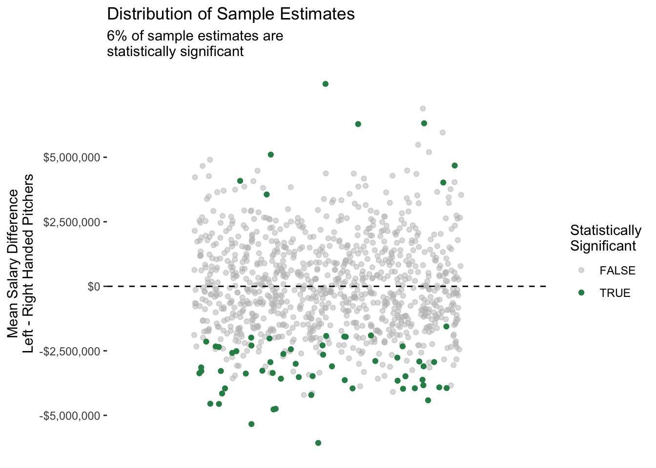
Our original result was really random noise: we happened by chance to draw a sample with some highly-paid left-handed pitchers!

This exercise illustrates what is known as the replication crisis: findings that are surprising in one sample may not hold in other repeated samples from the same population, or in the population as a whole. The replication crisis has many sources. One principal source is the one we illustrated above: sample-based estimates involve some randomness, and well-meaning researchers are (unfortunately) very good at telling interesting stories.

One solution to the replication crisis is to pay close attention to the statistical uncertainty in our estimates, such as that from random sampling. Another solution is to re-evaluate findings that are of interest on new samples. In any case, both the roots of the problem and the solutions are closely tied to sources of randomness in estimates, such as those generated using samples from a population.

The future of sample surveys

Sample surveys served as a cornerstone of social science research from the 1950s to the present. But there are concerns about their future:

some sampling frames, such as landline telephones, have become obsolete
response rates have been falling for decades
sample surveys are slower and more expensive than digital data

What is the future for sample surveys? How can they be combined with other data?

We will close with a discussion of these questions, which you can also engage with in the Groves 2011 reading that follows this module.

Using weights

When studying population-level inequality, our goal is to draw inference about all units in the population. We want to know about the people in the U.S., not just the people who answer the Current Population Survey. Drawing inference from a sample to a population is most straightforward for a simple random sample: when people are chosen at random with equal probabilities. For simple random samples, the sample average of any variable is an unbiased and consistent estimator of the population average.

But the Current Population Survey is not a simple random sample. Neither are most labor force samples! These samples still begin with a sampling frame, but people are chosen with unequal probabilities. We need sample weights to address this fact.

In the CPS, a key goal is to estimate unemployment in each state. Every state needs to have enough sample size—even tiny states like Wyoming. In order to make those estimates, the CPS oversamples people who live in small states.

An example: California and Wyoming

In 2022, California had 14,822 CPS-ASEC respondents out of a population of 39,029,342. Wyoming had 2,199 CPS-ASEC respondents out of 581,381 residents. The average probability that a CA resident was sampled was about 0.04 percent, whereas the same probability in WY was 0.4 percent. You are 10 times more likely to be sampled for the ASEC if you live in Wyoming.

To draw good population inference, our analysis must incorporate what we know about how the data were collected. If we ignore the weights, our sample will have too many people from Wyoming and too few people from California. Weights correct for this.

How survey designers create weights

To calculate sampling weight on person $i$, those who design survey samples take the ratio \[\text{weight on unit }i = \frac{1}{\text{probability of including person }i\text{ in the sample}}\] You can think of the sampling weight as the number of population members a given sample member represents. If there are 100 people with a 1% chance of inclusion, then on average 1 of them will be in the sample. That person represents $\frac{1}{.01}=100$ people.

Example redux: California and Wyoming

Suppose Californians are sampled with probability 0.0004. Then each Californian represents 1 / 0.0004 = 2,500 people. Each Californian should receive a weight of 2,500. Working out the same math for Wyoming, each Wyoming resident should receive a weight of 250. The total weight on these two samples will then be proportional to the sizes of these two populations.

In practice, weighting is more complicated: survey administrators adjust weights for differential nonresponse across population subgroups (a method called post-stratification). How to construct weights is beyond the scope of this course, and could be a whole course in itself!

Point estimates

When we download data, we typically download a column of weights. For simplicity, suppose we are given a sample of four people. The weight column tells us how many people in the population each person represents. The employed column tells us whether each person employed.

     name weight employed
1    Luis      4        1
2 William      1        0
3   Susan      1        0
4  Ayesha      4        1

If we take an unweighted mean, we would conclude that only 50% of the population is employed. But with a weighted mean, we would conclude that 80% of the population is employed! This might be the case if the sample was designed to oversample people at a high risk of unemployment.

Estimator	Math	Example	Result
Unweighted mean	$=\frac{\sum_{i=1}^n Y_i}{n}$	$=\frac{1 + 0 + 0 + 1}{4}$	= 50% employed
Weighted mean	$=\frac{\sum_{i=1}^n w_iY_i}{\sum_{i=1}^n w_i}$	$=\frac{41 + 10 + 10 + 41}{4 + 1 + 1 + 4}$	= 80% employed

In R, the weighted.mean(x, w) function will calculate weighted means where x is an argument for the outcome variable and w is an argument for the weight variable.

Standard errors

As you know from statistics, our sample mean is unlikely to equal the population mean. There is random variation in which people were chosen for inclusion in our sample, and this means that across hypothetical repeated samples we would get different sample means! You likely learned formulas to create a standard errors, which quantifies how much a sample estimator would move around across repeated samples.

Unfortunately, the formula you learned doesn’t work for complex survey samples! Simple random samples (for which those formulas hold) are actually quite rare. When you face a complex survey sample, those who administer the survey might provide

a vector of $n$ weights for making a point estimate
a matrix of $n\times k$ replicate weights for making standard errors

By providing $k$ different ways to up- and down-weight various observations, the replicate weights enable you to generate $k$ estimates that vary in a way that mimics how the estimator might vary if applied to different samples from the population. For instance, our employment sample might come with 3 replicate weights.

     name weight employed repwt1 repwt2 repwt3
1    Luis      4        1      3      5      3
2 William      1        0      1      2      2
3   Susan      1        0      3      1      1
4  Ayesha      4        1      5      3      4

The procedure to use replicate weights depends on how they are constructed. Often, it is relatively straightforward:

use weight to create a point estimate $\hat\tau$
use repwt* to generate $k$ replicate estimates $\hat\tau^*_1,\dots,\hat\tau^*_k$
calculate the standard error of $\hat\tau$ using the replicate estimates $\hat\tau^*$. The formula will depend on how the replicate weights were constructed, but it will likely involve the standard deviation of the $\hat\tau^*$ multiplied by some factor
construct a confidence interval² by a normal approximation \[(\text{point estimate}) \pm 1.96 * (\text{standard error estimate})\]

In our concrete example, the point estimate is 80% employed. The replicate estimates are 0.67, 0.73, 0.70. Variation across the replicate estimates tells us something about how the estimate would vary across hypothetical repeated samples from the population.

Computational strategy for replicate weights

Using replicate weights can be computationally tricky! It becomes much easier if you write an estimator() function. Your function accepts two arguments

data is the tibble containing the data
weight_name is the name of a column containing the weight to be used (e.g., “repwt1”)

Example. If our estimator is the weighted mean of employment,

estimator <- function(data, weight_name) {
  data |>
    summarize(
      estimate = weighted.mean(
        x = employed,
        # extract the weight column
        w = sim_rep |> pull(weight_name)
      )
    ) |> 
    # extract the scalar estimate
    pull(estimate)
}

In the code above, sim_rep |> pull(weight_name) takes the data frame sim_rep and extracts the weight variable that is named weight_name. There are other ways to do this also.

We can now apply our estimator to get a point estimate with the main sampling weight,

estimate <- estimator(data = sim_rep, weight_name = "weight")

which yields the point estimate 0.80. We can use the same function to produce the replicate estimates,

replicate_estimates <- c(
  estimator(data = sim_rep, weight_name = "repwt1"),
  estimator(data = sim_rep, weight_name = "repwt2"),
  estimator(data = sim_rep, weight_name = "repwt3")
)

yielding the three estimates: 0.67, 0.73, 0.70. In real data, you will want to apply this in a loop because there may be dozens of replicate weights.

The standard error of the estimator will be some function of the replicate estimates, likely involving the standard deviation of the replicate estimates. Check with the data distributor for a formula for your case. Once you estimate the standard error, a 95% confidence interval can be constructed with a Normal approximation, as discussed above.

Application in the CPS

Starting in 2005, the CPS-ASEC samples include 160 replicate weights. If you download replicate weights for many years, the file size will be enormous. We illustrate the use of replicate weights with a question that can be explored with only one year of data: among 25-year olds in 2023, how did the proportion holding four-year college degrees differ across those identifying as male and female?

We first load some packages, including the foreach package which will be helpful when looping through replicate weights.

library(tidyverse)
library(haven)
library(foreach)

To answer our research question, we download 2023 CPS-ASEC data including the variables sex, educ, age, the weight variable asecwt, and the replicate weights repwtp*.

cps_data <- read_dta("../data_raw/cps_00079.dta")

We then define an estimator to use with these data. It accepts a tibble data and a character weight_name identifying the name of the weight variable, and it returns a tibble with two columns: sex and estimate for the estimated proportion with a four-year degree.

estimator <- function(data, weight_name) {
  data |>
    # Define focal_weight to hold the selected weight
    mutate(focal_weight = data |> pull(weight_name)) |>
    # Restrict to those age 25+
    filter(age >= 25) |>
    # Restrict to valid reports of education
    filter(educ > 1 & educ < 999) |>
    # Define a binary outcome: a four-year degree
    mutate(college = educ >= 110) |>
    # Estimate weighted means by sex
    group_by(sex) |>
    summarize(estimate = weighted.mean(
      x = college,
      w = focal_weight
    ))
}

We produce a point estimate by applying that estimator with the asecwt.

estimate <- estimator(data = cps_data, weight_name = "asecwt")

# A tibble: 2 × 2
  sex        estimate
  <dbl+lbl>     <dbl>
1 1 [male]      0.369
2 2 [female]    0.397

Using the foreach package, we apply the estimator 160 times—once with each replicate weight—and use the argument .combine = "rbind" to stitch results together by rows.

library(foreach)
replicate_estimates <- foreach(r = 1:160, .combine = "rbind") %do% {
  estimator(data = cps_data, weight_name = paste0("repwtp",r))
}

# A tibble: 320 × 2
   sex        estimate
   <dbl+lbl>     <dbl>
 1 1 [male]      0.368
 2 2 [female]    0.396
 3 1 [male]      0.371
 4 2 [female]    0.400
 5 1 [male]      0.371
 6 2 [female]    0.397
 7 1 [male]      0.369
 8 2 [female]    0.397
 9 1 [male]      0.370
10 2 [female]    0.398
# ℹ 310 more rows

We estimate the standard error of our estimator by a formula \[\text{StandardError}(\hat\tau) = \sqrt{\frac{4}{160}\sum_{r=1}^{160}\left(\hat\tau^*_r - \hat\tau\right)^2}\] where the formula comes from the survey documentation. We carry out this procedure within groups defined by sex, since we are producing estimate for each sex.

standard_error <- replicate_estimates |>
  # Denote replicate estimates as estimate_star
  rename(estimate_star = estimate) |>
  # Merge in the point estimate
  left_join(estimate,
            by = join_by(sex)) |>
  # Carry out within groups defined by sex
  group_by(sex) |>
  # Apply the formula from survey documentation
  summarize(standard_error = sqrt(4 / 160 * sum((estimate_star - estimate) ^ 2)))

# A tibble: 2 × 2
  sex        standard_error
  <dbl+lbl>           <dbl>
1 1 [male]          0.00280
2 2 [female]        0.00291

Finally, we combine everything and construct a 95% confidence interval by a Normal approximation.

result <- estimate |>
  left_join(standard_error, by = "sex") |>
  mutate(ci_min = estimate - 1.96 * standard_error,
         ci_max = estimate + 1.96 * standard_error)

# A tibble: 2 × 5
  sex        estimate standard_error ci_min ci_max
  <dbl+lbl>     <dbl>          <dbl>  <dbl>  <dbl>
1 1 [male]      0.369        0.00280  0.364  0.375
2 2 [female]    0.397        0.00291  0.391  0.403

We use ggplot() to visualize the result.

result |>
  mutate(sex = as_factor(sex)) |>
  ggplot(aes(
    x = sex, 
    y = estimate,
    ymin = ci_min, 
    ymax = ci_max,
    label = scales::percent(estimate)
  )) +
  geom_errorbar(width = .2) +
  geom_label() +
  scale_x_discrete(
    name = "Sex", 
    labels = str_to_title
  ) +
  scale_y_continuous(name = "Proportion with 4-Year College Degree") +
  ggtitle(
    "Sex Disparities in College Completion",
    subtitle = "Estimates from the 2023 CPS-ASEC among those age 25+"
  )

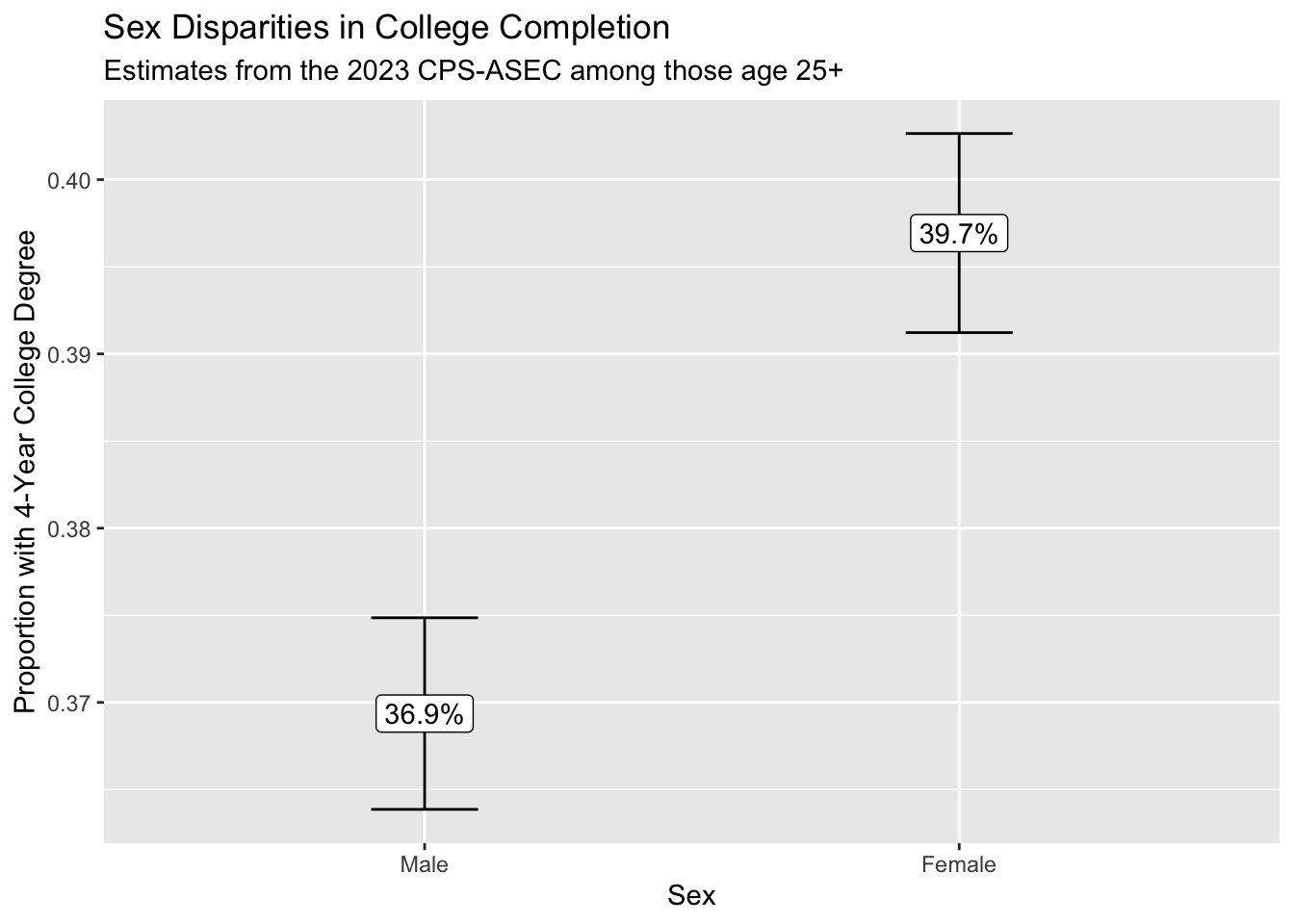
We conclude that those identifying as female are more likely to hold a college degree. Because we can see the confidence intervals generated using the replicate weights, we are reasonably confident in the statistical precision of our point estimates.

Takeaways

we use samples to learn about the population
this often requires sample weights because of unequal inclusion probabilities
point estimates are easy with functions like weighted.mean()
standard errors are harder, but possible via replicate weights
it can help to write an explicit estimator() function that carries out all the steps to estimate the unknown population parameters

At the highest level, it is important to remember that our goal is to study the population—not the sample. When we understand how the sample was generated from the population, this makes it possible to draw the correct inferences about the population from the sample.

Footnotes

Technically, a simple random sample draws units independently with equal probabilities, and with replacement. Our sample is actually drawn without replacement. In an infinite population, the two are equivalent.↩︎
If we hypothetically drew many complex survey samples from the population in this way, an interval generated this way would contain the true population mean 95% of the time.↩︎