population <- read_csv("https://soc114.github.io/data/baseball_population.csv")Logistic Regression
Logistic regression is an approach to predict binary outcomes (\(Y\) taking the values {0,1} or {FALSE,TRUE}) as a function of one or more predictor variables (a vector \(\vec{X}\)). This page introduces logistic regression using an example from the baseball data.
Baseball data example
As an example, we continue to use the data on baseball salaries, with a small twist. The file baseball_population.csv contains the following variables
playeris the player namesalaryis the 2023 salarypositionis the position played (e.g.,LHPfor left-handed pitcher)teamis the team nameteam_past_recordwas the team’s win percentage in the previous seasonteam_past_salarywas the team’s average salary in the previous season
A binary outcome
Suppose we model the probability that a player is a catcher (position == "C") as a linear function of player salary. For illustration, we do this on the full population.
ols_binary_outcome <- lm(
  position == "C" ~ salary,
  data = population
)
Catchers tend to have low salaries, so the probability of being a catcher declines as player salary rises. But the linear model carries this trend perhaps further than it ought to: the estimated probability of being a catcher for a player making $40 million is -2%! This prediction doesn’t make a lot of sense.
Code
population |>
  mutate(yhat = predict(ols_binary_outcome)) |>
  ggplot(aes(x = salary, y = yhat)) +
  geom_line() +
  geom_hline(yintercept = 0, linetype = "dashed") +
  scale_x_continuous(
    name = "Player Salary",
    labels = label_currency(scale = 1e-6, suffix = "m")
  ) +
  scale_y_continuous(
    name = "Predicted Probability\nof Being a Catcher"
  ) +
  theme_minimal() +
  ggtitle("Modeling a binary outcome with a line")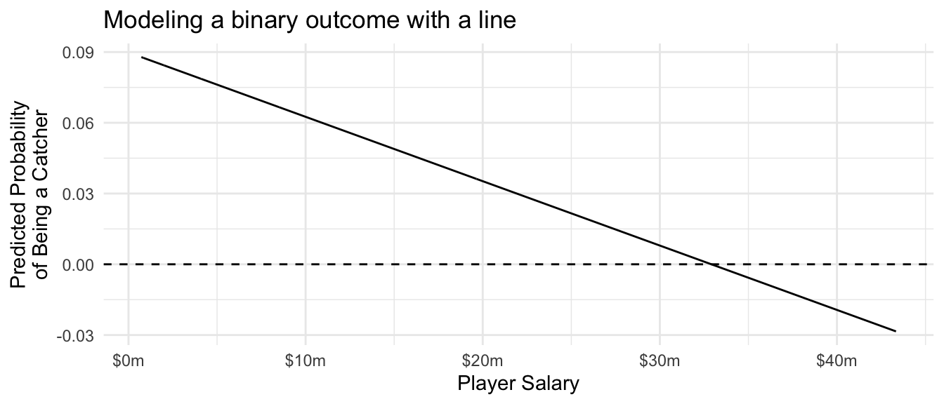
Logistic regression is similar to OLS, except that it uses a nonlinear function (the logistic function) to convert between coefficients that can take any negative or positive values and predictions that always fall in the [0,1] interval.
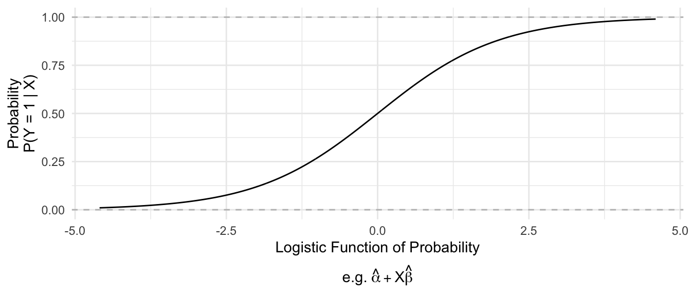
Mathematically, logistic regression replaces \(\text{E}(Y\mid\vec{X})\) on the left side of the equation with the logistic function.
\[ \underbrace{\log\left(\frac{\text{P}(Y\mid\vec{X})}{1 - \text{P}(Y\mid\vec{X})}\right)}_\text{Logistic Function} = \alpha + \vec{X}'\vec\beta \]
In our example with the catchers, we can use logistic regression to model the probability of being a catcher using the glm() function. The family = "binomial" line tells the function that we want to estimate logistic regression (since “binomial” is a distribution for outcomes drawn at random with a given probability).
logistic_regression <- glm(
  position == "C" ~ salary,
  data = population,
  family = "binomial"
)
We can predict exactly as with OLS, except that we need to add the type = "response" argument to ensure that R transforms the predicted values into the space of predicted probabilities [0,1] instead of the space in which the coefficients are defined (\(-\inf,\inf\)).
Code
population |>
  mutate(yhat = predict(logistic_regression, type = "response")) |>
  distinct(salary, yhat) |>
  ggplot(aes(x = salary, y = yhat)) +
  geom_line() +
  geom_hline(yintercept = 0, linetype = "dashed") +
  scale_x_continuous(
    name = "Player Salary",
    labels = label_currency(scale = 1e-6, suffix = "m")
  ) +
  scale_y_continuous(
    name = "Predicted Probability\nof Being a Catcher"
  ) +
  theme_minimal() +
  ggtitle("Modeling a binary outcome with logistic regression")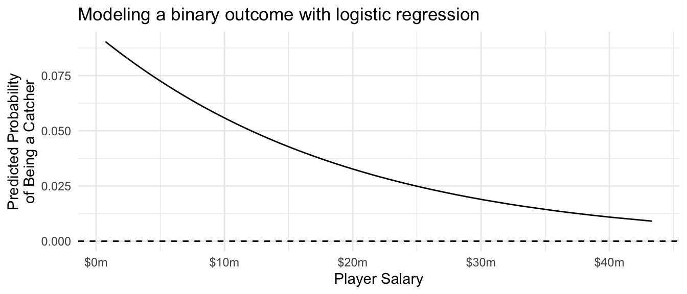
Predicting at new values
Suppose we had a new player whose salary was $5 million. What is the probability that this player is a catcher? We can define data at which to make a prediction.
to_predict <- tibble(salary = 5e6)Then we can predict, just as with OLS. Importantly, we use the type = "response" argument to specify that we want to predict the probability of being a catcher, not the log odds of being a catcher.
predict(
  logistic_regression,
  newdata = to_predict,
  type = "response"
)
1
0.07255671 What about a player with a salary of $40 million? With a salary so high, this player has a much lower probability of being a catcher.
to_predict_40 <- tibble(salary = 40e6)predict(
logistic_regression,
newdata = to_predict_40,
type = "response"
) 1
0.01090266 A player with a salary of $40 million has only a 1-in-100 chance of being a catcher, according to our model.
Comparison: Linear and logistic regression
To summarize, linear regression and logistic regression both use an assumed model to share information across units with different values of \(\vec{X}\). This model involves a linear predictor \(\hat\mu = \vec{X}'\hat{\vec\beta} = \hat\beta_0 + X_1\hat\beta_1 + X_2\hat\beta_2 + \cdots\).
The difference is that
- in OLS, the predicted value of \(Y\) is \(\hat\mu\)
- in logistic regression, the predicted value of \(Y\) is \(\text{logit}^{-1}(\hat\mu)\), which is a nonlinear function that ensures predicted values always fall between 0 and 1
In many practical settings, either OLS or logistic regression are good options with binary outcomes. The difference arises mainly when probabilities approach 0 and 1, in applications where it would be problematic to make predictions outside the (0,1) interval.