library(tidyverse)
motherhood_simulated <- read_csv("https://soc114.github.io/data/motherhood_simulated.csv")Problem Set 4: DAGs and Statistical Learning
Due: 5pm on Friday, Feb 28.
Student identifier: [type your anonymous identifier here]
The format of this problem set is different from the others.
- the assignment is a quiz in BruinLearn
- you will upload your PDF in that quiz
- you will also enter answer values in that quiz
The reason for this is that we are all busy with the final project! So you can have time for the project, there will be no peer review on this problem set. So the TAs can focus on helping with the project, some grading will be done automatically via the BruinLearn quiz.
Here is how to do this problem set:
- Use this pset4.qmd to complete the problem set.
- When you are finished, complete the quiz on BruinLearn
- you will upload your PDF there
- you will type some answers from your PDF there
1. (30 points) DAGs
For 1.1–1.5, answer True or False: \(X\) is a sufficient adjustment set to identify the causal effect of \(A\) on \(Y\). Recall that as you work on these problems, a good strategy is to first list all non-causal paths between \(A\) and \(Y\) and then cross out any that are blocked when conditioning on \(X\).
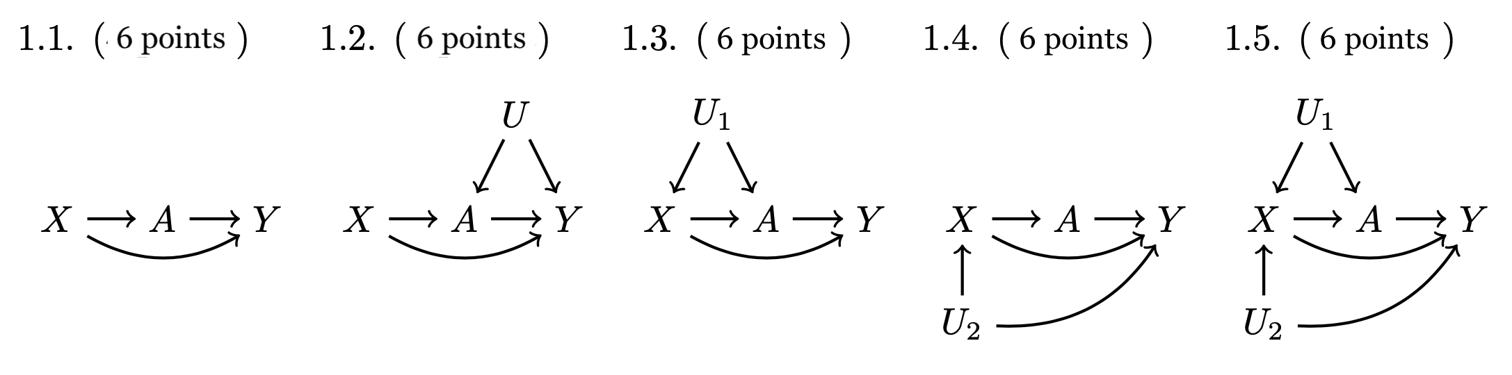
1.1. [answer here]
1.2. [answer here]
1.3. [answer here]
1.4. [answer here]
1.5. [answer here]
2. Causal inference with statistical modeling
The paragraphs below introduce this part of the problem set. Your work begins at “Prepare your data.”
How does parenthood affect labor market outcomes? For an outcome \(Y\) such as employment, we can imagine that each person \(i\) has a potential outcome as a parent \(Y_i^1\) and a potential outcome as a non-parent, \(Y_i^0\). Parenthood casually shapes an outcome like employment to the degree that these differ.
The effect of parenthood on labor market outcomes has been the subject of extensive social science research which has revealed a consistent finding: parenthood may improve men’s labor market outcomes while harming women’s labor market outcomes (e.g., Waldfogel 1998, Budig & England 2001, Correll et al. 2007). The disparate effects of parenthood for men and women are thus one source of gender disparities in labor market outcomes.
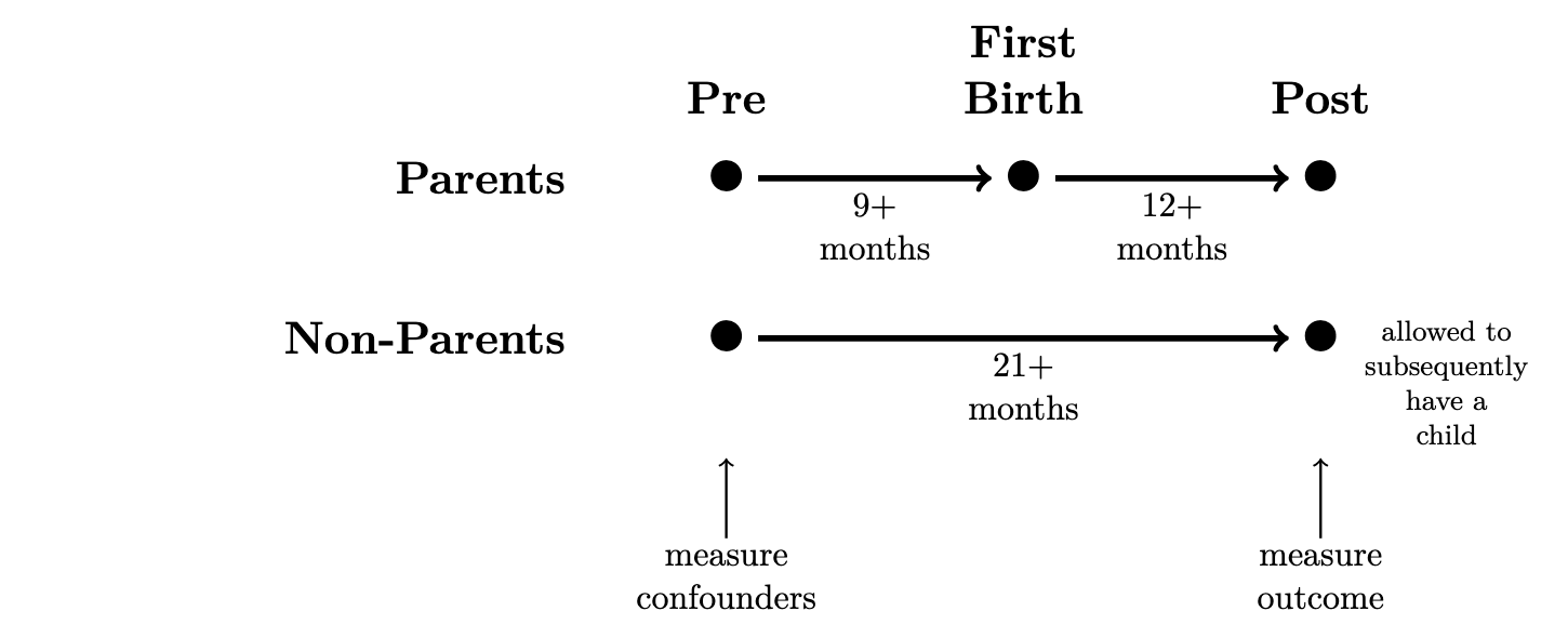
This problem set estimates the causal effect of motherhood on mothers’ employment, using data simulated to approximate data that exist in the National Longitudinal Survey of Youth 1997 cohort. The NLSY97 interviews people repeatedly across years. We manipulated these data so that each row contains information from a pre- and a post-observation, separated by 21+ months. In the pre-observation, we measure confounding variables. In the post-observation, we measure the outcome (y, employment). Between the pre- and post-observation, some women experience a first birth (treated == TRUE) and others do not (treated == FALSE).
The dataset motherhood_simulated.csv contains the following variables.
observation_idis an index for each observationsampling_weightis the weight due to unequal probability samplingtreatedindicates a first birth (TRUEorFALSE)- This occurred between the pre- and post-periods.
yis the outcome, codedTRUEif employed orFALSEif not employed.- This was measured in the post-period.
The data include a set of variables measured in the pre-period. We will consider these to be a sufficient adjustment set. These were measured in the pre-period.
raceis a categorical variable codedHispanic,Non-Hispanic Black, andNon-Hispanic Non-Blackpre_ageis age in yearspre_educis an ordinal variable for educational attainment, codedLess than high school,High school,2-year degree, and4-year degreewith those with higher levels of education also coded in this last categorypre_maritalis a categorical variable of marital status, codedno_partner,cohabiting, ormarriedpre_employedis a lag measure of employment in the prior survey wave, codedTRUEandFALSEpre_fulltimeindicates full-time employment in the prior survey wave, codedTRUEandFALSEpre_tenureis years of experience with a current employer, as of the prior survey wavepre_experienceis total years of full-time work experience, as of the prior survey wave
Prepare your data
Filter to create two data objects: one with mothers who have treated == TRUE and one with non-mothers who have treated == FALSE.
# your code hereEstimate by linear model predictions
Among non-mothers, model the probability of employment with a linear model. As predictors, use an additive function of the sufficient adjustment set.
Hints:
- Use the
lm()function. - use this model formula:
y ~ race + pre_age + pre_educ + pre_marital + pre_employed + pre_fulltime + pre_tenure + pre_experience - for the
dataargument, use your data containing non-mothers. - you will need the argument
weights = sampling_weightto specify to weight the model by thesampling_weightvariable
# your code here2.1. (10 points) Report a predicted value
Using your model estimated among non-mothers, make predictions of \(\hat{Y}^0\) among mothers. Report the predicted value for the first mother in the data.
Hints:
- Use
predict()to make predictions. - We suggest your store the variables in a new variable in your dataset using
mutate(). - To see the first predicted value in your predicted data, one strategy is to use
select()to keep only the variable you’ve created that contains your predicted value.
# your code here2.2. (10 points) Report an ATT estimate
Across mothers, estimate the Average Treatment Effect on the Treated (ATT) by the weighted mean difference between \(Y\) (observed) and \(\hat{Y}^0\) (predicted from linear regression), weighted by sampling weights.
- For each mother, take the difference between the observed outcome
yand the probability of employment that you predict for her in the absence of motherhood. - Then take the weighted mean across mothers weighted by the sampling weight.
- Report this weighted mean.
# your code here