What is a model?

This is the second part of lecture for Feb 11. Slides are here

What is a model, and why would we use one? This page introduces ideas with two models: Ordinary Least Squares and logistic regression.

At a high level, a model is a tool to share information across units with different \(\vec{X}\) values when estimating subgroup summaries, such as the conditional mean \(\text{E}(Y\mid\vec{X} = \vec{x})\) within the subgroup taking predictor value \(\vec{X} = \vec{x}\). By assuming that this conditional mean follows a particular shape defined by a small number of parameters, models can yield better predictions than the sample subgroup means. The advantages of models are particularly apparent when there aren’t very many units observed in each subgroup.

Later in the course, we will expand our conception of models to include flexible statistical learning procedures. For now, we will focus on two models from classical statistics.

A simple example

As an example, we continue to use the data on baseball salaries, with a small twist. The file baseball_population.csv contains the following variables

population <- read_csv("https://soc114.github.io/data/baseball_population.csv")

• player is the player name
• team is the team name
• salary is the 2023 salary
• team_past_record is the 2022 proportion of games won by that team
• team_past_salary is the 2022 mean salary in that team

Our goal: using a sample, estimate the mean salary of all Dodger players in 2023. Because we have the population, we know the true mean is $6.23m. We will imagine that we don’t know this number. Instead of having the full population, we will imagine we have

• information on predictors for all players: position, team, team past record
• information on salary for a random sample of 5 players per team

Our estimation task will be made difficult by a lack of data: we will work with a sample containing many teams (30), and few players per team (5). We will use statistical learning strategies to pool information from those other teams’ players to help us make a better estimate of the Dodger mean salary.

Our predictor will be the team_past_salary from the previous year. We assume that a team’s past salary in 2022 tells us something about their mean salary in 2023.

For illustration, draw a sample of 5 players per team

sample <- population |>
  group_by(team) |>
  sample_n(5) |>
  ungroup()

Construct a tibble with the observations to be predicted: the Dodgers.

to_predict <- population |>
  filter(team == "L.A. Dodgers")

Ordinary Least Squares

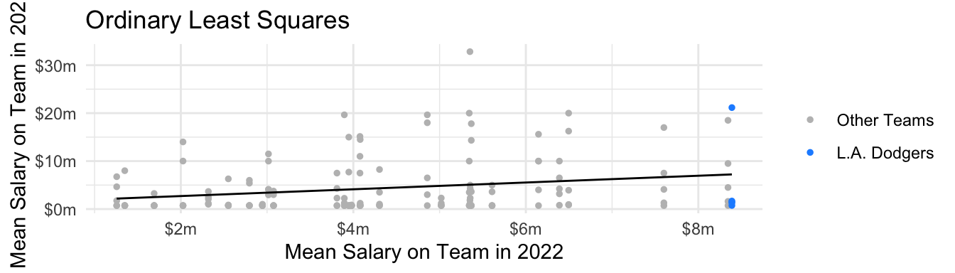
We could model salary next year as a linear function of team past salary by Ordinary Least Squares. In math, OLS produces a prediction \[\hat{Y}_i = \hat\alpha + \hat\beta X_i\] with \(\hat\alpha\) and \(\hat\beta\) chosen to minimize the sum of squared errors, \(\sum_{i=1}^n \left(Y_i - \hat{Y}_i\right)^2\). Visually, it minimizes all the line segments below.

Here is how to estimate an OLS model using R.

model <- lm(salary ~ team_past_salary, data = sample)

Then we could predict the mean salary for the Dodgers.

predicted <- to_predict |>
  mutate(predicted = predict(model, newdata = to_predict))

We would report the mean predicted salary for the Dodgers.

predicted |>
  summarize(estimated_Dodger_mean = mean(predicted))

# A tibble: 1 × 1
  estimated_Dodger_mean
                  <dbl>
1              7224025.

Our model-based estimate compares to the true population mean of $6.23m.

Logistic regression

Sometimes the outcome is binary (taking the values {0,1} or {FALSE,TRUE}). One can model binary outcomes with linear regression, but sometimes the predicted values are negative or greater than 1. As an example, suppose we model the probability that a player is a Designated Hitter (position == "DH") as a linear function of player salary. For illustration, we do this on the full population.

ols_binary_outcome <- lm(
  position == "C" ~ salary,
  data = population
)

Catchers tend to have low salaries, so the probability of being a catcher declines as player salary rises. But the linear model carries this trend perhaps further than it ought to: the estimated probability of being a catcher for a player making $40 million is -2%! This prediction doesn’t make a lot of sense.

population |>
  mutate(yhat = predict(ols_binary_outcome)) |>
  ggplot(aes(x = salary, y = yhat)) +
  geom_line() +
  geom_hline(yintercept = 0, linetype = "dashed") +
  scale_x_continuous(
    name = "Player Salary",
    labels = label_currency(scale = 1e-6, suffix = "m")
  ) +
  scale_y_continuous(
    name = "Predicted Probability\nof Being a Catcher"
  ) +
  theme_minimal() +
  ggtitle("Modeling a binary outcome with a line")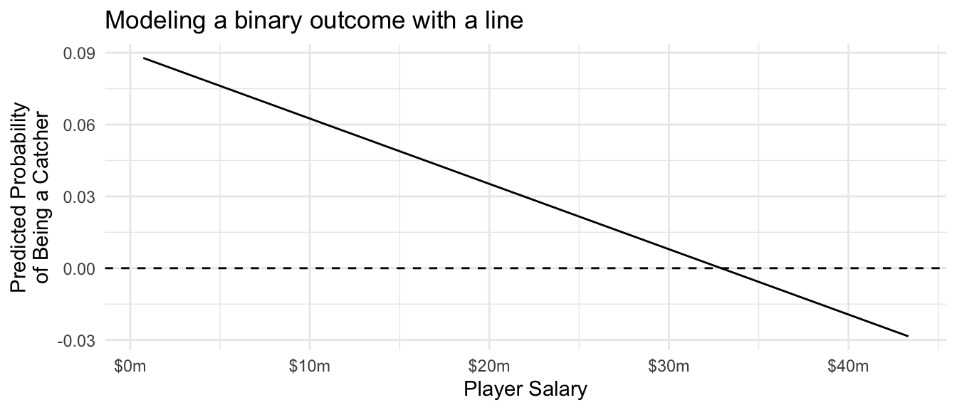

Logistic regression is simialr to OLS, except that it uses a nonlinear function (the logistic function) to convert between coefficients that can take any negative or positive values and predictions that always fall in the [0,1] interval.

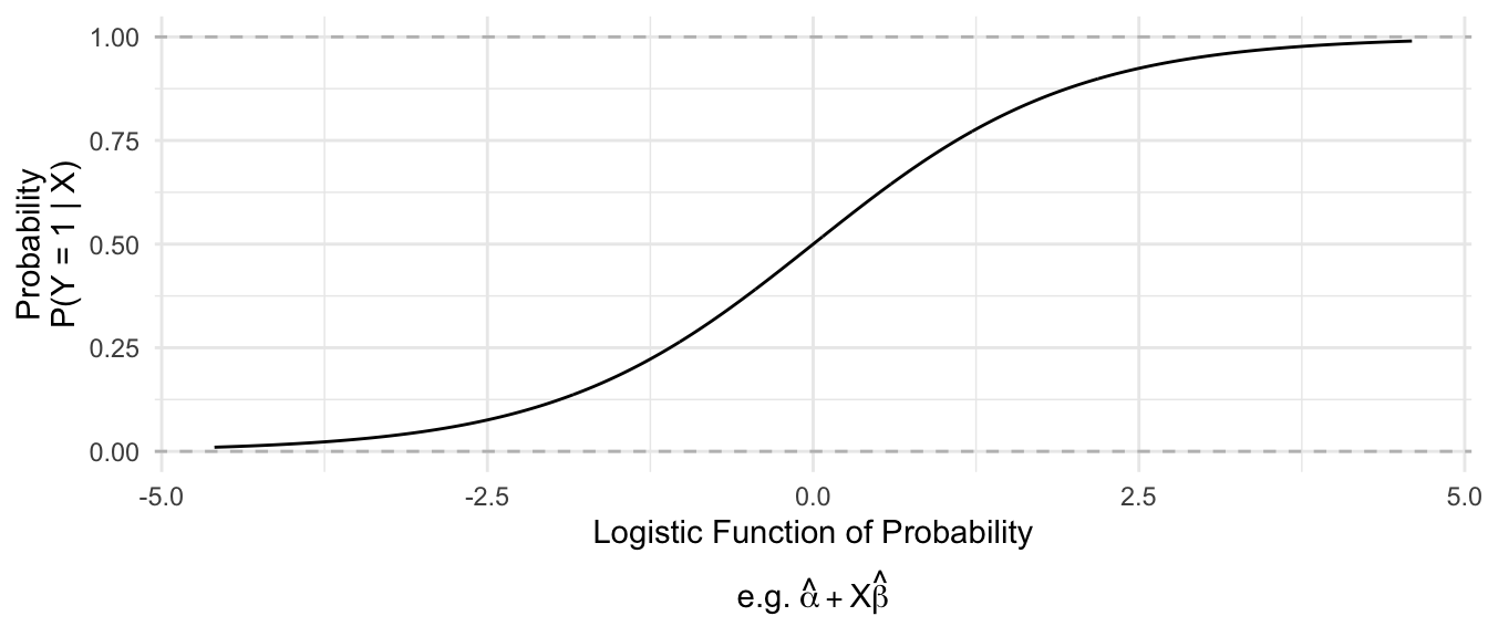
Mathematically, logistic regression replaces \(\text{E}(Y\mid\vec{X})\) on the left side of the equation with the logistic function.

\[ \underbrace{\log\left(\frac{\text{P}(Y\mid\vec{X})}{1 - \text{P}(Y\mid\vec{X})}\right)}_\text{Logistic Function} = \alpha + \vec{X}'\vec\beta \]

In our example with the catchers, we can use logistic regression to model the probability of being a catcher using the glm() function. The family = "binomial" line tells the function that we want to estimate logistic regression (since “binomial” is a distribution for outcomes drawn at random with a given probability).

logistic_regression <- glm(
  position == "C" ~ salary,
  data = population,
  family = "binomial"
)

We can predict exactly as with OLS, except that we need to add the type = "response" argument to ensure that R transforms the predicted values into the space of predicted probabilities [0,1] instead of the space in which the coefficients are defined (\(-\inf,\inf\)).

population |>
  mutate(yhat = predict(logistic_regression, type = "response")) |>
  distinct(salary, yhat) |>
  ggplot(aes(x = salary, y = yhat)) +
  geom_line() +
  geom_hline(yintercept = 0, linetype = "dashed") +
  scale_x_continuous(
    name = "Player Salary",
    labels = label_currency(scale = 1e-6, suffix = "m")
  ) +
  scale_y_continuous(
    name = "Predicted Probability\nof Being a Catcher"
  ) +
  theme_minimal() +
  ggtitle("Modeling a binary outcome with logistic regression")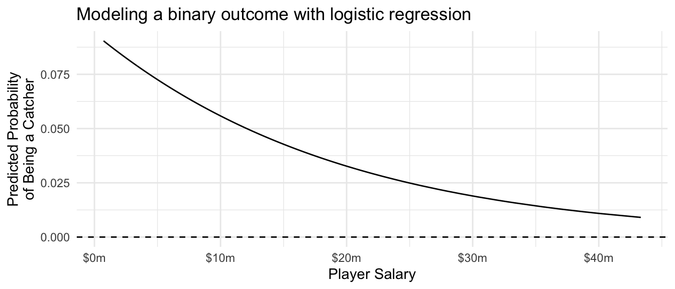

Below is code to make a prediction for the L.A. Dodgers.

predicted_logistic <- predict(
  logistic_regression,
  newdata = to_predict,
  type = "response"
)

To summarize, linear regression and logistic regression both use an assumed model to share information across units with different values of \(\vec{X}\) when estimating \(\text{E}(Y\mid \vec{X})\) or \(\text{P}(Y = 1\mid\vec{X})\). This is especially useful any time when we do not get to observe many units at each value of \(\vec{X}\).