Directed Acyclic Graphs
This topic is covered Feb 6. Here are slides.
Directed Acyclic Graphs (DAGs) formalize causal assumptions mathematically in graphs. One way DAGs are useful in observational studies is by helping us to identify a sufficient adjustment set (\(\vec{X}\)) such that conditional exchangeability holds.
Nodes, edges, and paths
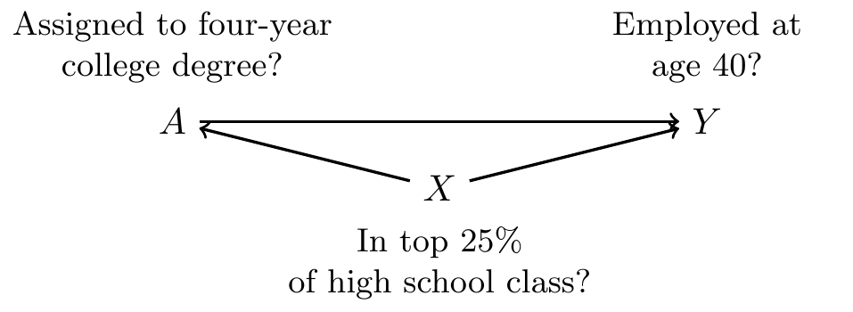
The previous page introduced a conditionally randomized experiment in which the researcher assigned participants to the treatment condition of (four-year college degree) vs (high school degree) with probabilities that depended on high school class rank. In this experiment, being in the top 25% of one’s high school class caused a higher chance of receiving the treatment. We will also assume that both high school performance and college completion may causally shape employment at age 40.
We can formalize these ideas in a graph where each node (a letter) is a variable and each edge (\(\rightarrow\)) is a causal relationship.
Between each pair of nodes, you can enumerate every path or sequence of edges connecting the nodes.
Path. A path between nodes \(A\) and \(B\) is any set of edges that starts at \(A\) and ends at \(B\). Paths can involve arrows in either direction.
In our DAG above, there are two paths between \(A\) and \(Y\).
- \(A\rightarrow Y\)
- \(A\leftarrow X \rightarrow Y\)
We use paths to determine the reasons why \(A\) and \(Y\) might be statistically dependent or independent.
Causal paths
The first type of path that we consider is a causal path.
Causal path. A path in which all arrows point in the same direction. For example, \(A\) and \(D\) could be connected by a causal path \(A\rightarrow B \rightarrow C \rightarrow D\).
A causal path creates statistical depends between the nodes because the first node causes the last node, possibly through a sequence of other nodes.
In our example, there is a causal path \(A\rightarrow Y\): being assigned to a four-year college degree affects employment at age 40. Because of this causal path, people who are assigned to a four-year degree have different rates of employment at age 40 than those who are not.
A causal path can go through several variables. For example, if we listed the paths between \(X\) and \(Y\) we would include the path \(X\rightarrow A \rightarrow Y\). This is a causal path because being in the top 25% of one’s high school class increases the probability of assignment to a four-year degree in our experiment, which in turn increases the probability of employment at age 40.
Fork structures
To reason about non-causal paths, we have to think about several structures that can exist along these paths. The first such structure is a fork structure.
Fork structure. A fork structure is a sequence of edges in which two variables (\(A\) and \(B\)) are both caused a third variable (\(C\)): \(A\leftarrow C \rightarrow B\).
In our example, the path \(A\leftarrow X \rightarrow Y\) involves a fork structure. being in the top 25% of one’s high school class causally affects both the treatment (college degree) and the outcome (employment at age 40).
A fork structure creates statistical dependence between \(A\) and \(Y\) that does not correspond to a causal effect of \(A\) on \(Y\). In our example, people who are assigned to the treatment value (college degree) are more likely to have been in the top 25% of their high school class, since this high class rank affected treatment assignment in our experiment. A high class rank also affected employment at age 40. Thus, in our experiment the treatment would be associated with the outcome even if finishing college had no causal effect on employment.
Fork structures can be blocked by conditioning on the common cause. In our example, suppose we filter our data to only include those in the top 25% of their high school class. We sometimes use a box to denote conditioning on a variable, (\(A\leftarrow\boxed{X}\rightarrow Y\)). Conditioning on \(X\) blocks the path because within this subgroup \(X\) does not vary, so it cannot cause the values of \(A\) and \(Y\) within the subgroup. In our example, if we looked among those in the top 25% of their high school classes the only reason college enrollment would be related to employment at age 40 would be the causal effect \(A\rightarrow Y\).
To emphasize ideas, it is also helpful to consider a fork structure in an example where the variables have no causal relationship.
Suppose a beach records for each day the number of ice cream cones sold and the number of rescues by lifeguards. There is no causal effect between these two variables; eating ice cream does not cause more lifeguard rescues and vice versa. But the two are correlated because they share a common cause: warm temperatures cause high ice cream sales and also high lifeguard rescues. A fork structure formalizes this notion: \((\text{ice cream sales}) \leftarrow (\text{warm temperature}) \rightarrow (\text{lifeguard rescues})\).
In the population of days as a whole, this fork structure means that ice cream sales are related to lifeguard rescues. But if we condition on having a warm temperature by filtering to days when the temperature took a particular value, ice cream sales would be unrelated to lifeguard rescues across those days. This is the sense in which conditioning on the common cause variable blocks the statistical associations that would otherwise arise from a fork structure.
Collider structures
In contrast to a fork structure where one variable affects two others (\(\bullet\leftarrow\bullet\rightarrow\bullet\)), a collider structure is a structure where one variable is affected by two others.
Collider structure. A collider structure is a sequence of edges in which two variables (\(A\) and \(B\)) both cause a third variable (\(C\)). We say that \(C\) is a collider on the path \(A\rightarrow C \leftarrow B\).
Fork and collider structures have very different properties, as we will illustrate through an example.
Suppose that every day I observe whether the grass on my lawn is wet. I have sprinklers that turn on with a timer at the same time every day, regardless of the weather. It also sometimes rains. When the grass is wet, it is wet because either the sprinklers have been on or it has been raining.
\[ (\text{sprinklers on}) \rightarrow (\text{grass wet}) \leftarrow (\text{raining}) \]
If I look across all days, the variable (sprinklers on) is unrelated to the variable (raining). After all, the sprinklers are just on a timer! Formally, we say that even though (sprinklers on) and (raining) are connected by the path above, this path is blocked by the collider structure. A path does not create dependence between two variables when it contains a collider structure.
If I look only at the days when the grass is wet, a different pattern emerges. If the grass is wet and the sprinklers have not been on, then it must have been raining: the grass had to get wet somehow. If the grass is wet and it has not been raining, then the sprinklers must have been on. Once I look at days when the grass is wet (or condition on the grass being wet), the two input variables become statistically associated.
A collider blocks a path when that collider is left unadjusted, but conditioning on the collider variable opens the path containing the collider.
Open and blocked paths
A central purpose of a DAG is to connect causal assumptions to implications about associations that should be present (or absent) in data under those causal assumptions. To make this connection, we need a final concept of open and blocked paths.
A path is blocked if it contains an unconditioned collider or a conditioned non-collider. Otherwise, the path is open. An open path creates statistical dependence between its terminal nodes whereas a blocked path does not.
As examples for a path with no colliders,
- \(A\leftarrow B \rightarrow C \rightarrow D\) is an open path because no variables are conditioned and it contains no colliders.
- \(A\leftarrow \boxed{B}\rightarrow C \rightarrow D\) is a blocked path because we have conditioned on the non-collider \(B\).
- \(A\leftarrow B\rightarrow \boxed{C} \rightarrow D\) is a blocked path because we have conditioned on the non-collider \(C\).
Determining statistical dependence
We are now ready to use DAGs to determine if \(A\) and \(B\) are statistically dependent. The process involves three steps.
- List all paths between \(A\) and \(B\).
- Cross out any paths that are blocked.
- The causal assumptions imply that \(A\) and \(B\) may be statistically dependent only if any open paths remain.
As an example, below we consider a hypothetical DAG.

1. Marginal dependence
Marginally without any adjustment, are \(A\) and \(D\) statistically dependent? We first write out all paths connecting \(A\) and \(D\).
- \(A\rightarrow B \leftarrow C\rightarrow D\)
- \(A\leftarrow X\rightarrow D\)
We then cross out the paths that are blocked
- \(\cancel{A\rightarrow B \leftarrow C\rightarrow D}\) (blocked by unconditioned collider \(B\))
- \(A\leftarrow X\rightarrow D\)
Because an open path remains, \(A\) and \(D\) are statistically dependent.
2. Dependence conditional on \(X\)
If we condition on \(X\), are \(A\) and \(D\) statistically dependent? We first write out all paths connecting \(A\) and \(D\).
- \(A\rightarrow B \leftarrow C\rightarrow D\)
- \(A\leftarrow \boxed{X}\rightarrow D\)
We then cross out the paths that are blocked
- \(\cancel{A\rightarrow B \leftarrow C\rightarrow D}\) (blocked by unconditioned collider \(B\))
- \(\cancel{A\leftarrow \boxed{X}\rightarrow D}\) (blocked by conditioned non-collider \(X\))
Because no open path remains, \(A\) and \(D\) are statistically independent.
3. Dependence conditional on \(\{X,B\}\)
If we condition on \(X\) and \(B\), are \(A\) and \(D\) statistically dependent? We first write out all paths connecting \(A\) and \(D\).
- \(A\rightarrow B \leftarrow C\rightarrow D\)
- \(A\leftarrow \boxed{X}\rightarrow D\)
We then cross out the paths that are blocked
- \(A\rightarrow \boxed{B} \leftarrow C\rightarrow D\) (open since collider \(B\) is conditioned)
- \(\cancel{A\leftarrow \boxed{X}\rightarrow D}\) (blocked by conditioned non-collider \(X\))
Because an open path remains, \(A\) and \(D\) are statistically dependent.
Causal identification with DAGs
When our aim is to identify the average causal effect of \(A\) on \(Y\), we want to choose a set of variables for adjustment so that all remaining paths are causal paths. We call this a sufficient adjustment set.
A sufficient adjustment set for the causal effect of \(A\) on \(Y\) is a set of nodes that, when conditioned, block all non-causal paths between \(A\) and \(Y\).
In our example from the top of this page, there were two paths between \(A\) and \(Y\):
- \((A\text{: college degree})\rightarrow (Y\text{: employed at age 40})\)
- \((A\text{: college degree})\leftarrow (X\text{: top 25\% of high school class})\rightarrow (Y\text{: employed at age 40})\)
In this example, \(X\) is a sufficient adjustment set. Once we condition on \(X\) by e.g. filtering to those in the top 25% of their high school class, the only remaining path between \(A\) and \(Y\) is the causal path \(A\rightarrow Y\). Thus, the difference in means in \(Y\) across \(A\) within subgroups defined by \(X\) identifies the conditional average causal effect of \(A\) on \(Y\).
A more difficult example.
Sufficient adjustment sets can be much more complicated. As an example, consider the DAG below.
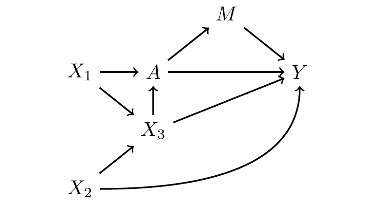
We first list all paths between \(A\) and \(Y\).
- \(A\rightarrow Y\)
- \(A\rightarrow M\rightarrow Y\)
- \(A\leftarrow X_1\rightarrow X_3 \rightarrow Y\)
- \(A\leftarrow X_1\rightarrow X_3 \leftarrow X_2\rightarrow Y\)
- \(A\leftarrow X_3 \rightarrow Y\)
- \(A\leftarrow X_3\leftarrow X_2 \rightarrow Y\)
The first two paths are causal, and the others are non-causal. We want to find a sufficient adjustment set to block all the non-causal paths.
In order to block paths (3), (5), and (6) we might condiiton on \(X_3\). But doing so opens path (2), which was otherwise blocked by the collider \(X_3\). In order to also block path (2), we might additionally condition on \(X_1\). In this case, our sufficient adjustment set is \(\{X_1,X_3\}\).
- \(A\rightarrow Y\)
- \(A\rightarrow M\rightarrow Y\)
- \(\cancel{A\leftarrow \boxed{X_1}\rightarrow \boxed{X_3} \rightarrow Y}\)
- \(\cancel{A\leftarrow \boxed{X_1}\rightarrow \boxed{X_3} \leftarrow X_2\rightarrow Y}\)
- \(\cancel{A\leftarrow \boxed{X_3} \rightarrow Y}\)
- \(\cancel{A\leftarrow \boxed{X_3}\leftarrow X_2 \rightarrow Y}\)
Then the only open paths are paths (1) and (2), both of which are causal paths from \(A\) to \(Y\).
Sometimes there are several sufficient adjustment sets. In this example, sufficient adjustment sets include:
- \(\{X_1,X_3\}\)
- \(\{X_2,X_3\}\)
- \(\{X_1,X_2,X_3\}\)
We sometimes call the first two minimal sufficient adjustment sets because they are the smallest.
A minimal sufficient adjustment set is an adjustment set that achieves causal identification by conditioning on the fewest number of variables possible.
How to draw a DAG
So far, we have focused on causal identification with a DAG that has been given. But how do you draw one for yourself?
When drawing a DAG, there is an important rule: any node that would have edges pointing into any two nodes already represented in the DAG must be included. This is because what you omit from the DAG is far more important than what you include in the DAG. Many of your primary assumptions are about the nodes and edges that you leave out.
For example, suppose we are estimating the causal effect of a college degree on employment at age 40. After beginning our DAG with only these variables, we have to think about any other variables that might affect these two. High school performance is one example. Then we have to include any nodes that affect any two of {high school performance, college degree, employment at age 40}. Perhaps a person’s parents’ education affects that person’s high school performance and college degree attainment. Then parents’ education should be included as an additional node. The cycle continues, so that in observational causal inference settings you are likely to have a DAG with many nodes.
In practice, you may not have data on all the nodes that comprise the sufficient adjustment set in your graph. In this case, we recommend that you first draw a graph under which you can form a sufficient adjustment set with the measured variables. This allows you to state one set of causal beliefs under which your analysis can answer your causal question. Then, also draw a second DAG that includes the other variables you think are relevant. This will enable you to reason about the sense in which your results could be misleading because of omitting important variables.
Closing thoughts
DAGs are a powerful tool for causal inference, because they are both visually intuitive and mathematically precise. They translate our theories about the world into a formal language with implications for causal identification.
If you’d like to learn more about DAGs, here are a few good resources:
- Pearl, Judea, and Dana Mackenzie. 2018. The Book of Why: The New Science of Cause and Effect. New York: Basic Books.
- Pearl, Judea, Madelyn Glymour, and Nicholas P. Jewell. 2016. Causal Inference in Statistics: A Primer. New York: Wiley.