Regression models perform well when the the response surface \(E(Y\mid\vec{X})\) follows a line (or some other assumed shape). In some settings, however, the response surface may be more complex. There may be nonlinearities and interaction terms that the researcher may not know about in advance. In these settings, one might desire an estimator that adaptively learns the functional form from the data. Trees are one such approach.
A simulation to illustrate trees
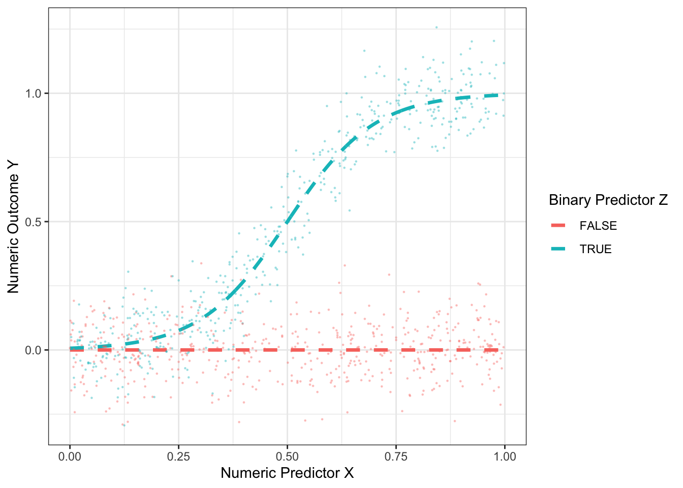
As an example, the figure below presents some hypothetical data with a binary predictor \(Z\), a numeric predictor \(X\), and a numeric outcome \(Y\).
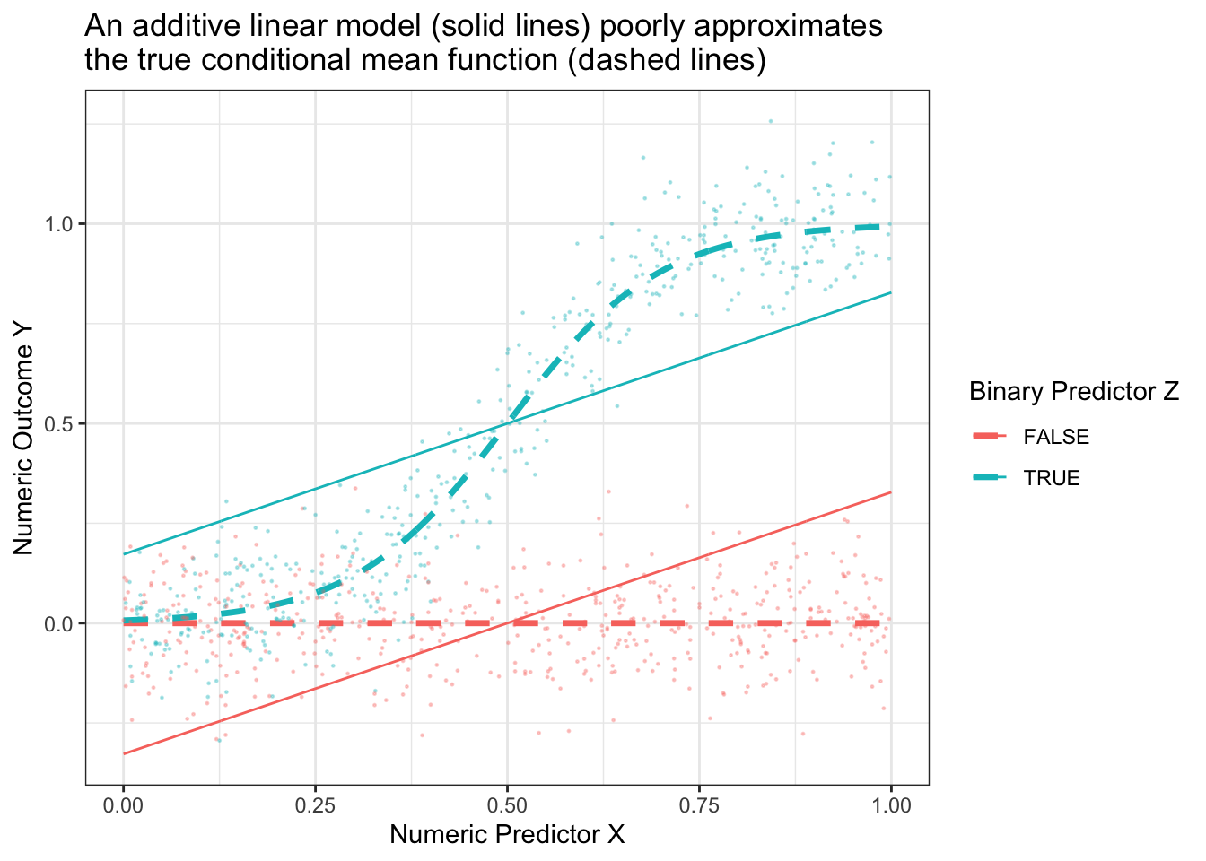
If we tried to approximate these conditional means with an additive linear model, \[\hat{E}_\text{Linear}(Y\mid X,Z) = \hat\alpha + \hat\beta X + \hat\gamma Z\] then the model approximation error would be very large.
Code
best_linear_fit <-lm(mu ~ x + z, data = true_conditional_mean)p +geom_line(data = true_conditional_mean |>mutate(mu =predict(best_linear_fit)) ) +theme_bw() +ggtitle("An additive linear model (solid lines) poorly approximates\nthe true conditional mean function (dashed lines)")
How a tree works
A regression tree begins from a radically different place than regression. Instead of assuming that the response follows some assumed pattern, trees proceed by a much more inductive process: recursive splits.
Trees repeatedly split the data
With no model at all, suppose we were to split the sample into two subgroups. For example, we might choose to split on \(Z\) and say that all units with z = TRUE are one subgroup while all units with z = FALSE are another subgroup. Or we might split on \(X\) and say that all units with x <= .23 are one subgroup and all units with x > .23 are another subgroup. After choosing a way to split the dataset into two subgroups, we would then make a prediction rule: for each unit, predict the mean value of all sampled units who fall in their subgroup. This rule would produce only two predicted values: one prediction per resulting subgroup.
If you were designing an algorithm to predict this way, how would you choose to define the split?
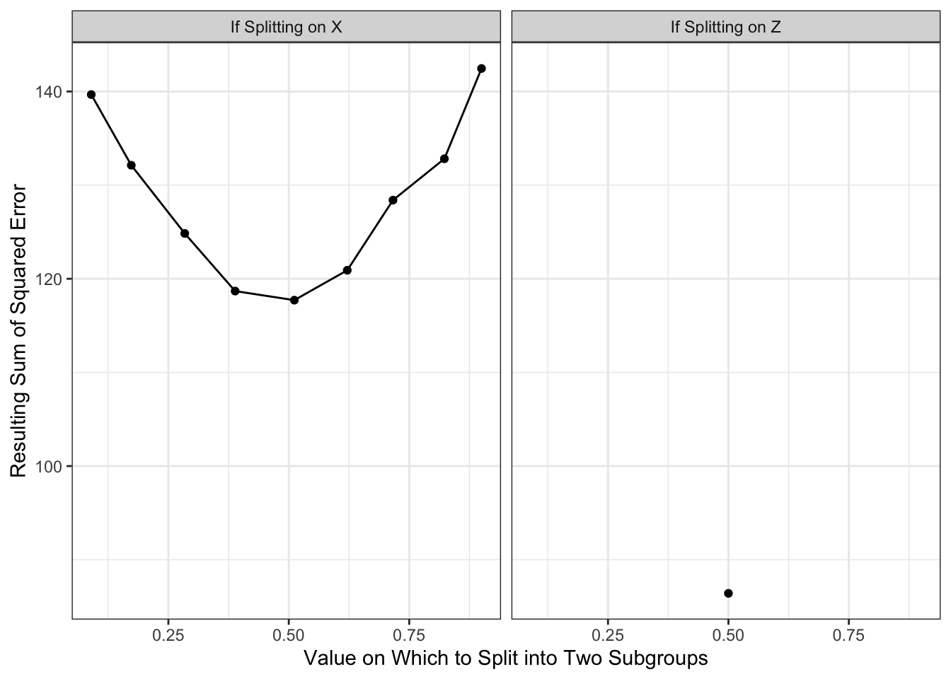
In regression trees to estimate conditional means, the split is often chosen to minimize the resulting sum of squared prediction errors. Suppose we choose this rule. Suppose we consider splitting on \(X\) being above or below each decile of its empirical distribution. Suppose we consider splitting on \(Z\) being FALSE or TRUE. The graph below shows the sum of squared prediction error resulting from each rule.
Code
x_split_candidates <-quantile(simulated_data$x, seq(.1,.9,.1))z_split_candidates <- .5by_z <- simulated_data |>group_by(z) |>mutate(yhat =mean(y)) |>ungroup() |>summarize(sum_squared_error =sum((yhat - y) ^2))by_x <-foreach(x_split = x_split_candidates, .combine ="rbind") %do% { simulated_data |>mutate(left = x <= x_split) |>group_by(left) |>mutate(yhat =mean(y)) |>ungroup() |>summarize(sum_squared_error =sum((yhat - y) ^2)) |>mutate(x_split = x_split)}by_x |>mutate(split ="If Splitting on X") |>rename(split_value = x_split) |>bind_rows( by_z |>mutate(split ="If Splitting on Z") |>mutate(split_value = .5) ) |>ggplot(aes(x = split_value, y = sum_squared_error)) +geom_point() +geom_line() +facet_wrap(~split) +labs(x ="Value on Which to Split into Two Subgroups",y ="Resulting Sum of Squared Error" ) +theme_bw()
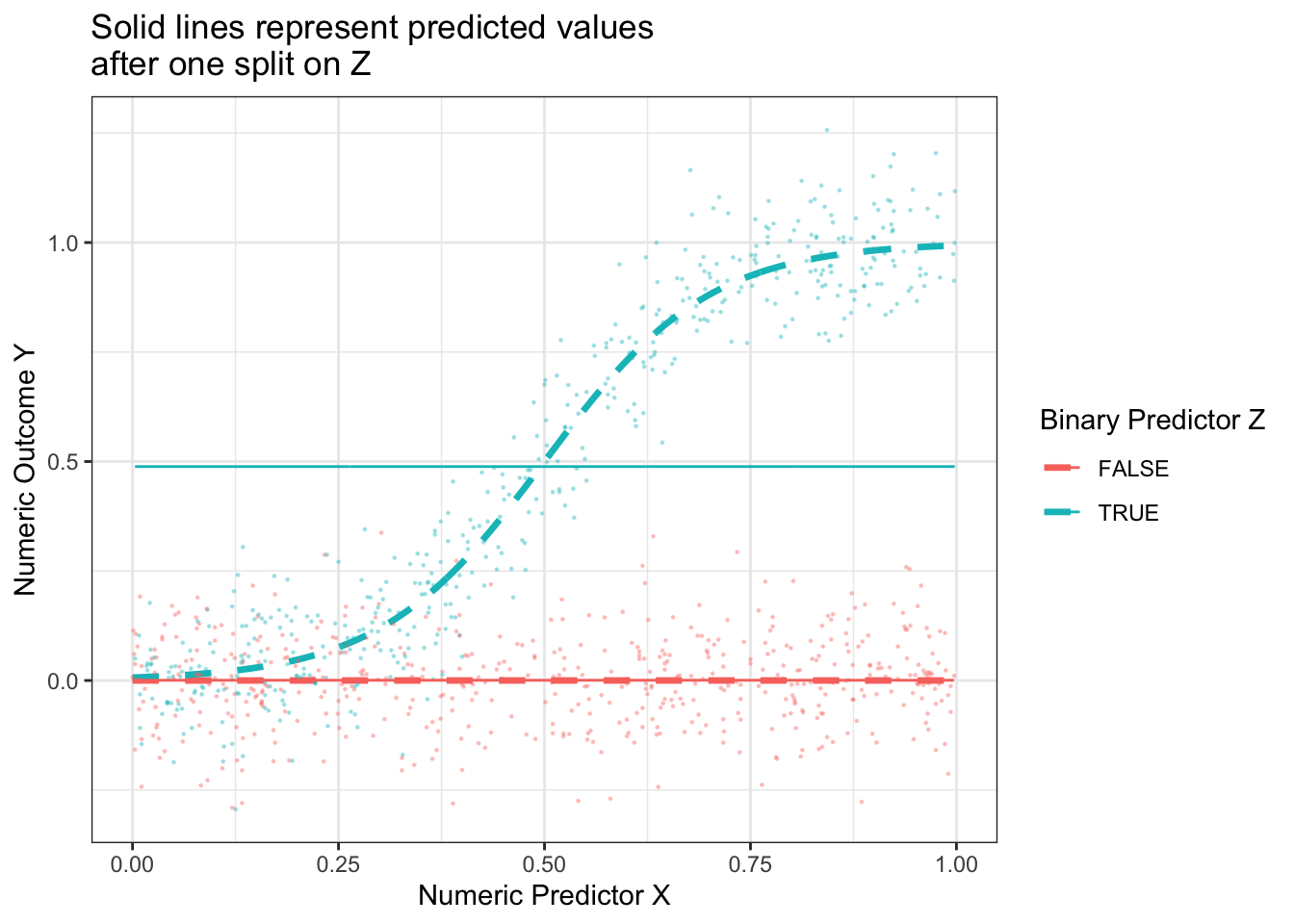
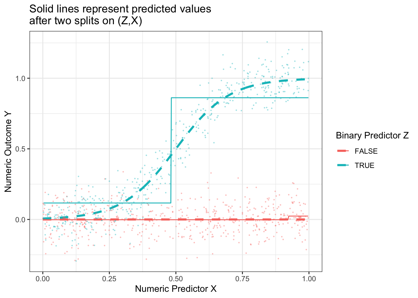
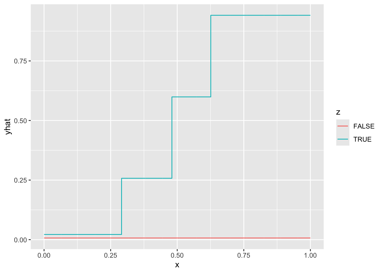
With the results above, we would choose to split on \(Z\), creating a subpopulation with \(Z \leq .5\) and a subgroup with \(Z\geq .5\). Our prediction function would look like this. Our split very well approximates the true conditional mean function when Z = FALSE, but is still a poor approximator when Z = TRUE.
Code
p +geom_line(data = simulated_data |>group_by(z) |>mutate(mu =mean(y)) ) +ggtitle("Solid lines represent predicted values\nafter one split on Z")
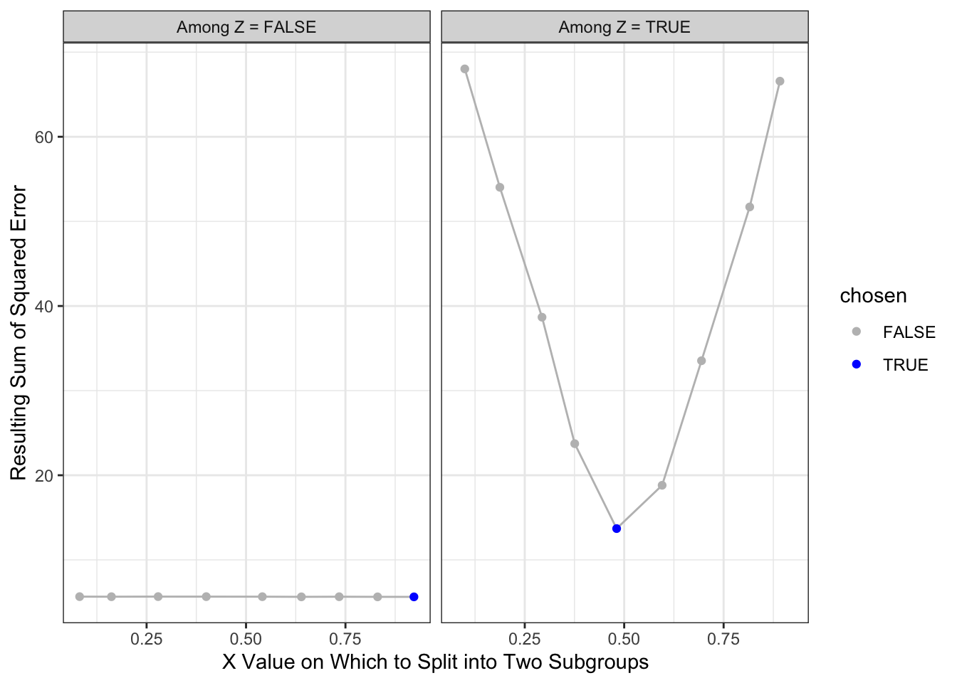
What if we make a second split? A regression tree repeats the process and considers making a further split within each subpopulation. The graph below shows the sum of squared error in the each subpopulation of Z when further split at various candidate values of X.
Code
# Split 2: After splitting by Z, only X remains on which to splitleft_side <- simulated_data |>filter(!z)right_side <- simulated_data |>filter(z)left_split_candidates <-quantile(left_side$x, seq(.1,.9,.1))right_split_candidates <-quantile(right_side$x, seq(.1,.9,.1))left_split_results <-foreach(x_split = left_split_candidates, .combine ="rbind") %do% { left_side |>mutate(left = x <= x_split) |>group_by(z,left) |>mutate(yhat =mean(y)) |>ungroup() |>summarize(sum_squared_error =sum((yhat - y) ^2)) |>mutate(x_split = x_split)} |>mutate(chosen = sum_squared_error ==min(sum_squared_error))right_split_results <-foreach(x_split = right_split_candidates, .combine ="rbind") %do% { right_side |>mutate(left = x <= x_split) |>group_by(z,left) |>mutate(yhat =mean(y)) |>ungroup() |>summarize(sum_squared_error =sum((yhat - y) ^2)) |>mutate(x_split = x_split)} |>mutate(chosen = sum_squared_error ==min(sum_squared_error))split2_results <- left_split_results |>mutate(split1 ="Among Z = FALSE") |>bind_rows(right_split_results |>mutate(split1 ="Among Z = TRUE"))split2_results |>ggplot(aes(x = x_split, y = sum_squared_error)) +geom_line(color ='gray') +geom_point(aes(color = chosen)) +scale_color_manual(values =c("gray","blue")) +facet_wrap(~split1) +theme_bw() +labs(x ="X Value on Which to Split into Two Subgroups",y ="Resulting Sum of Squared Error" )
The resulting prediction function is a step function that begins to more closely approximate the truth.
Code
split2_for_graph <- split2_results |>filter(chosen) |>mutate(z =as.logical(str_remove(split1,"Among Z = "))) |>select(z, x_split) |>right_join(simulated_data, by =join_by(z)) |>mutate(x_left = x <= x_split) |>group_by(z, x_left) |>mutate(yhat =mean(y))p +geom_line(data = split2_for_graph,aes(y = yhat) ) +ggtitle("Solid lines represent predicted values\nafter two splits on (Z,X)")
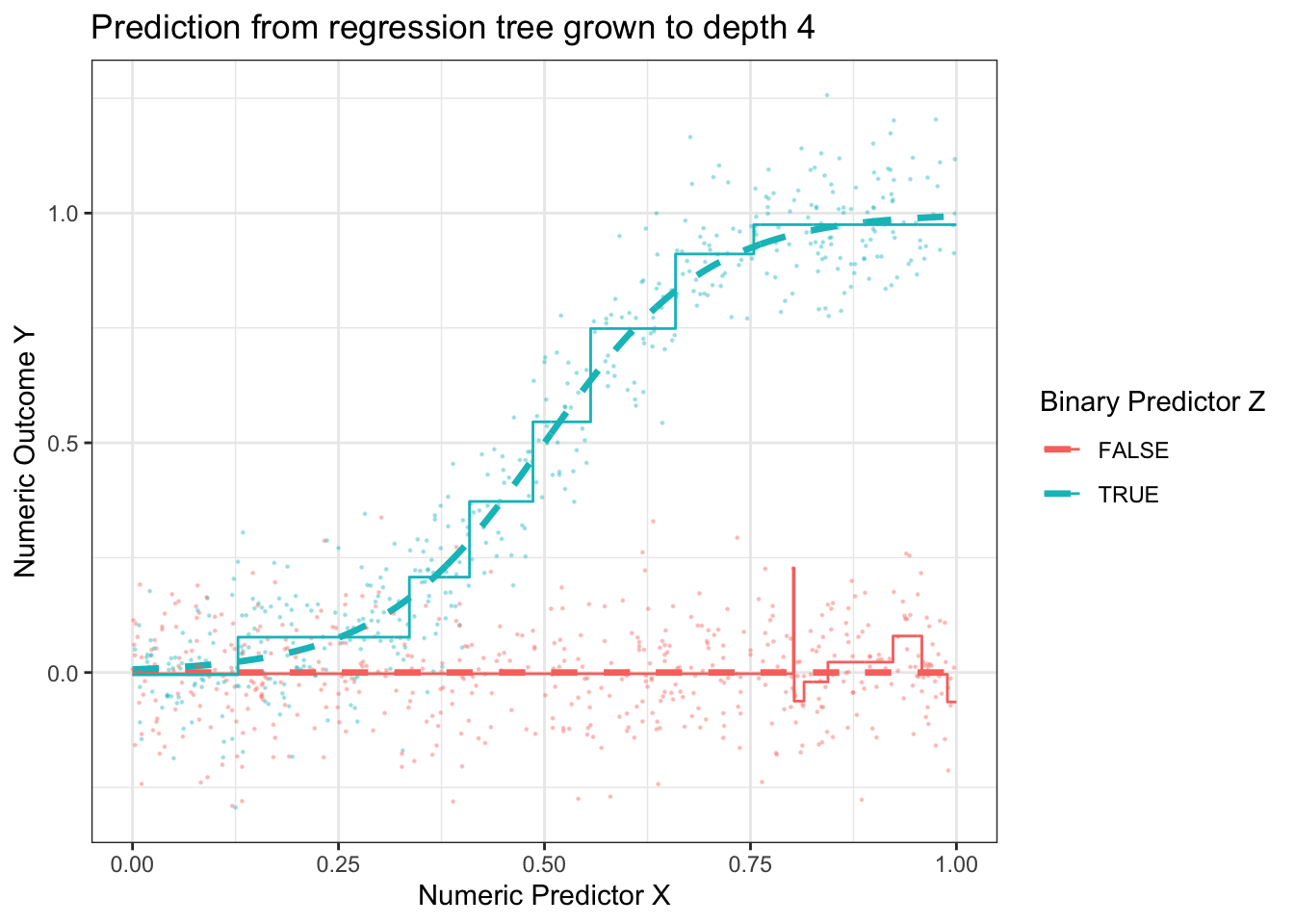
Having made one and then two splits, the figure below shows what happens when each subgroup is the created by 4 sequential splits of the data.
Code
library(rpart)rpart.out <-rpart( y ~ x + z, data = simulated_data, control =rpart.control(minsplit =2, cp =0, maxdepth =4))p +geom_step(data = true_conditional_mean |>mutate(mu_hat =predict(rpart.out, newdata = true_conditional_mean)),aes(y = mu_hat) ) +ggtitle("Prediction from regression tree grown to depth 4")
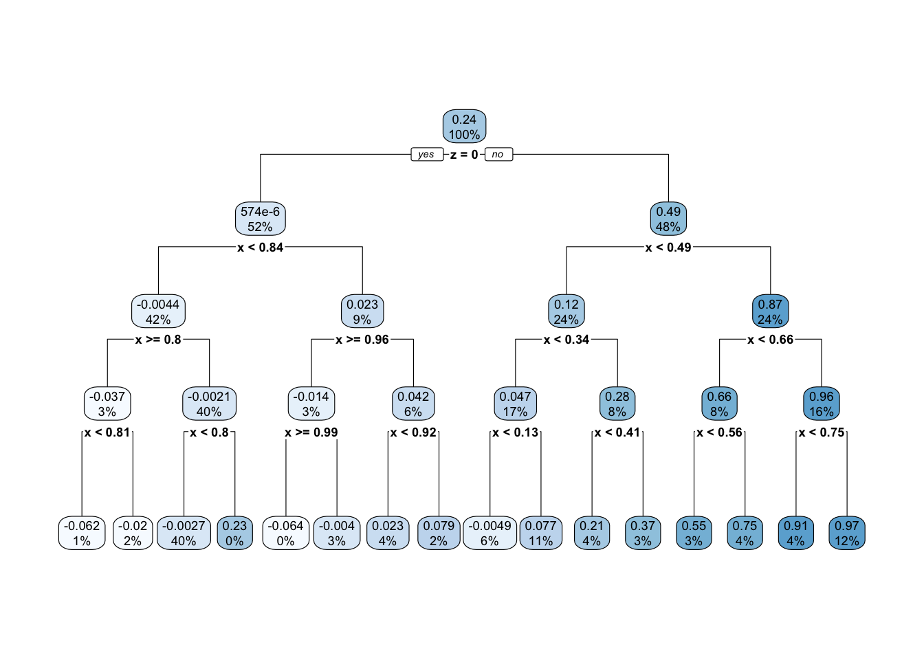
This prediction function is called a regression tree because of how it looks when visualized a different way. One begins with a full sample which then “branches” into a left and right part, which further “branch” off in subsequent splits. The terminal nodes of the tree—subgroups defined by all prior splits—are referred to as “leaves.” Below is the prediction function from above, visualized as a tree. This visualization is made possible with the rpart.plot package which we practice further down the page.
Try different specifications of the tuning parameters. See the control argument of rpart, explained at ?rpart.control. To produce a model with depth 4, we previously used the argument control = rpart.control(minsplit = 2, cp = 0, maxdepth = 4).
Tuning parameter: Depth
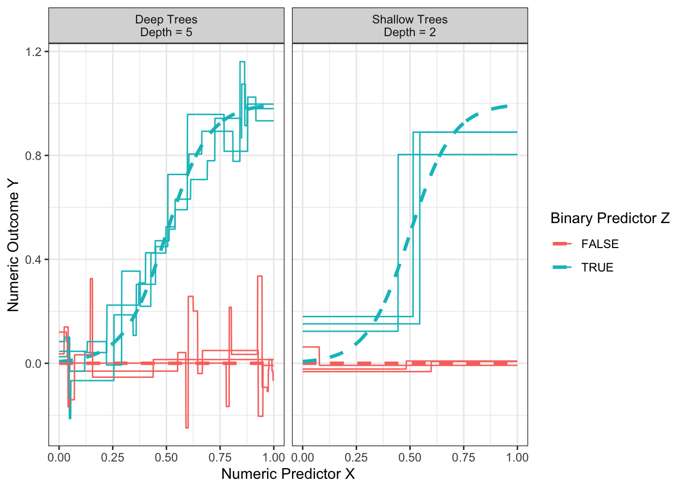
How deep should one make a tree? Recall that the depth of the tree is the number of sequential splits that define a leaf. The figure below shows relatively shallow trees (depth = 2) and relatively deep trees (depth = 4) learned over repeated samples. What do you notice about performance with each choice?
Shallow trees yield predictions that tend to be more biased because the terminal nodes are large. At the far right when z = TRUE and x is large, the predictions from the shallow trees are systematically lower than the true conditional mean.
Deep trees yield predictions that tend to be high variance because the terminal nodes are small. While the flexibility of deep trees yields predictions that are less biased, the high variance can make deep trees poor predictors.
The balance between shallow and deep trees can be chosen by various rules of thumb or out-of-sample performance metrics, many of which are built into functions like rpart. Another way out is to move beyond trees to forests, which involve a simple extension that yields substantial improvements in performance.