library(tidyverse)
motherhood_simulated <- read_csv("https://soc114.github.io/data/motherhood_simulated.csv")Problem Set 8: Matching
For this problem set, the Gradescope submission system will have you enter an answer for every question. The last question will ask you to upload your code file. There are two parts: conceptual questions and coding questions. You will submit all parts in a single Gradescope assignment.
Conceptual questions
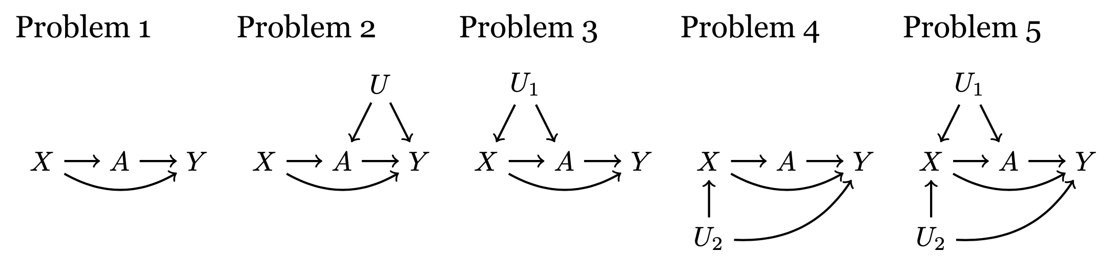
For 1.1–1.5, answer True or False: if we compared treated units (\(A = 1\)) to a matched set of untreated units (\(A = 0\)) who were identical on \(X\), we would identify the average treatment effect on the treated. Recall that a good strategy is to first list all paths between \(A\) and \(Y\), cross out any that are blocked when conditioning on \(X\), and then determine whether all open paths are causal paths. See the DAGs course page for help.
TODO Renumber to 1 to 5.
Coding part
The paragraphs below introduce the data we will use. Your work begins at “Load the data.”
How does parenthood affect labor market outcomes? For an outcome \(Y\) such as employment, we can imagine that each person \(i\) has a potential outcome as a parent \(Y_i^1\) and a potential outcome as a non-parent, \(Y_i^0\). Parenthood causally shapes an outcome like employment to the degree that these differ.
The effect of parenthood on labor market outcomes has been the subject of extensive social science research which has revealed a consistent finding: parenthood may improve men’s labor market outcomes while harming women’s labor market outcomes (e.g., Waldfogel 1998, Budig & England 2001, Correll et al. 2007). The disparate effects of parenthood for men and women are thus one source of gender disparities in labor market outcomes.
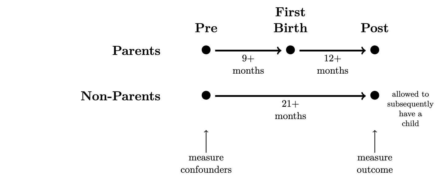
This problem set estimates the causal effect of motherhood on mothers’ employment, using data simulated to approximate data that exist in the National Longitudinal Survey of Youth 1997 cohort. The NLSY97 interviews people repeatedly across years. We manipulated these data so that each row contains information from a pre- and a post-observation, separated by 21+ months. In the pre-observation, we measure confounding variables. In the post-observation, we measure the outcome (y, employment). Between the pre- and post-observation, some women experience a first birth (treated == TRUE) and others do not (treated == FALSE).
The dataset motherhood_simulated.csv contains the following variables.
observation_idis an index for each observationsampling_weightis the weight due to unequal probability samplingtreatedindicates a first birth (TRUEorFALSE)- This occurred between the pre- and post-periods.
yis the outcome, codedTRUEif employed orFALSEif not employed.- This was measured in the post-period.
The data include a set of variables measured in the pre-period. We will consider these to be a sufficient adjustment set. These were measured in the pre-period.
raceis a categorical variable codedHispanic,Non-Hispanic Black, andNon-Hispanic Non-Blackpre_ageis age in yearspre_educis an ordinal variable for educational attainment, codedLess than high school,High school,2-year degree, and4-year degreewith those with higher levels of education also coded in this last categorypre_maritalis a categorical variable of marital status, codedno_partner,cohabiting, ormarriedpre_employedis a lag measure of employment in the prior survey wave, codedTRUEandFALSEpre_fulltimeindicates full-time employment in the prior survey wave, codedTRUEandFALSEpre_tenureis years of experience with a current employer, as of the prior survey wavepre_experienceis total years of full-time work experience, as of the prior survey wave
Load the data
You can load the data with the code below.
We will use these data to estimate the average causal effect of motherhood on employment among mothers. This estimand is the average treatment effect on the treated. \[ \text{E}(Y^1-Y^0\mid A = 1) \]
We will carry out estimation by 1:1 nearest neighbor matching on the estimated propensity score.
- There are 1,815 treated observations and 19,379 untreated observations in the data. After 1:1 matching for the ATT, how many treated observations will there be?
- After 1:1 matching for the ATT, how many untreated observations will there be?
Load the MatchIt package. Within this package, use the matchit function to carry out 1:1 nearest neighbor matching on the propensity score. Our in-class example illustrates how to use this function on a different dataset. For the formula argument, use this model formula which says to model the log odds of treatment as an additive function of all confounders.
treated ~ race + pre_age + pre_educ +
    pre_marital + pre_employed + pre_fulltime +
    pre_tenure + pre_experience
Use the summary() function on the object you created with matchit() to see the distribution of confounding variables in the full data and in the matched data.
- What is the mean age of non-mothers in the full data?
- What is the mean age of non-mothers in the matched data?
- The mean age of non-mothers is more similar to the mean age of mothers in (a) the full data or (b) the matched data?
Use match_data() to extract the matches from the output of your call to matchit(). Among the matches, summarize the unweighted mean value of y within groups defined by treated. If you need help with this look back at where you estimated subgroup means in Problem Set 2.
- Based on your estimate, what proportion of mothers would be employed if they were counterfactually not parents?
- Based on your estimate, what is the average causal effect of motherhood on employment, among mothers in this sample?