Data Example
This page provides a concrete example of observational causal inference. We will use this example to learn matching and models for causal inference.
Motivating question
To what extent does completing a four-year college degree by age 25 increase the probability of having a spouse or residential partner with a four-year college degree at age 35, among the population of U.S. residents who were ages 12–16 at the end of 1996?
This causal question draws on questions in sociology and demography about assortative mating: the tendency of people with high education, income, or status to form households together1. One reason to care about assortative mating is that it can contribute to inequality across households: if people with high earnings potential form households together, then income inequality across households will be greater than it would be if people formed households randomly.
Our question is causal: to what extent is the probability of marrying a four-year college graduate higher if one were hypothetically to finish a four-year degree, versus if that same person were hypothetically to not finish a college degree?
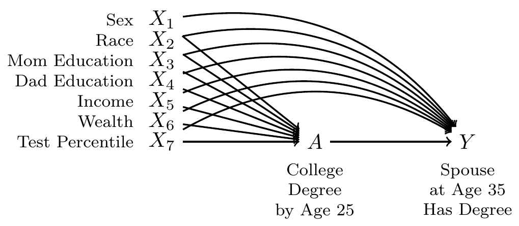
In data that exist in the world, we see only one of these two potential outcomes. The people for whom we see the outcome under a college degree are systematically different from those for whom we see the outcome under no degree: college graduates come from families with higher incomes, higher wealth, and higher parental education, for example. All of these factors may directly shape the probability of marrying a college graduate even in the absence of college. Thus, it will be important to adjust for a set of measured confounders, represented by \(\vec{X}\) in our DAG.
By adjusting for the variables \(\vec{X}\), we block all non-causal paths between the treatment \(A\) and the outcome \(Y\) in the DAG. If this DAG is correct, then conditional exchangeability holds with this adjustment set: \(\{Y^1,Y^0\}\unicode{x2AEB} A \mid\vec{X}\).
To estimate, we use data from the National Longitudinal Survey of Youth 1997, a probability sample of U.S. resident children who were ages 12–16 on Dec 31, 1996. The study followed these children and interviewed them every year through 2011 and then every other year after that.
We will analyze a simulated version of these data (nlsy97_simulated.csv), which you can access with this line of code.
data <- read_csv("https://soc114.github.io/data/nlsy97_simulated.csv")
Expand to learn how to get the actual data
To access the actual data, you would need to register for an account, log in, upload the nlsy97.NLSY97 tagset that identifies our variables, and then download. Unzip the folder and put the contents in a directory on your computer. Then run our code file prepare_nlsy97.R in that folder. This will produce a new file d.RDS, contains the data. You could analyze that file. In the interest of transparency, we wrote the code nlsy97_simulated.R to convert these real data to simulated data that we can share.
The data contain several variables
idis an individual identifier for each personais the treatment, containing the respondent’s education codedtreatedif the respondent completed a four-year college degree anduntreatedif not.yis the outcome:TRUEif has a spouse or residential partner at age 35 who holds a college degree, andFALSEif no spouse or partner or if the spouse or partner at age 35 does not have a degree.- There are several pre-treatment variables
sexis codedFemaleandMaleraceis race/ethnicity and is codedHispanic,Non-Hispanic Black, andNon-Hispanic Non-Black.mom_educis the respondent’s mother’s education as reported in 1997. It takes the valueNo momif the child had no residential mother in 1997, and otherwise is coded with her education:< HS,High school,Some college, orCollege.dad_educis the respondent’s father’s education as reported in 1997. It takes the valueNo dadif the child had no residential father in 1997, and otherwise is coded with his education:< HS,High school,Some college, orCollege.log_parent_incomeis the log of gross household income in 1997log_parent_wealthis the log of household net worth in 1997test_percentileis the respondent’s percentile score on a test of math and verbal skills administered in 1999 (the Armed Services Vocational Aptitude Battery).
When values are missing, we have replcaed them with predicted values. In the simulated data, no row represents a real person because values have been drawn randomly from a probability distribution designed to mimic what exists in the real data. As discussed above, we did this in order to share the file with you by a download on this website.
Footnotes
For reviews, see Mare 1991 and Schwartz 2013.↩︎